A simple simulation example

George G Vega Yon

February 25, 2019

R Markdown

Step 1: Loading the packages

library(netdiffuseR)
library(sna)

Step 2: Random network (for input)

set.seed(8826)

# Simulating a small world (10, 3) with pr = .3
net <- rgraph_ws(50, 3, .3)

# A bit more of rewiring
net <- rewire_graph(net, p=3, both.ends = TRUE)

## Warning in rewire_graph(net, p = 3, both.ends = TRUE): The option -copy.first-
## is set to TRUE. In this case, the first graph will be treated as a baseline,
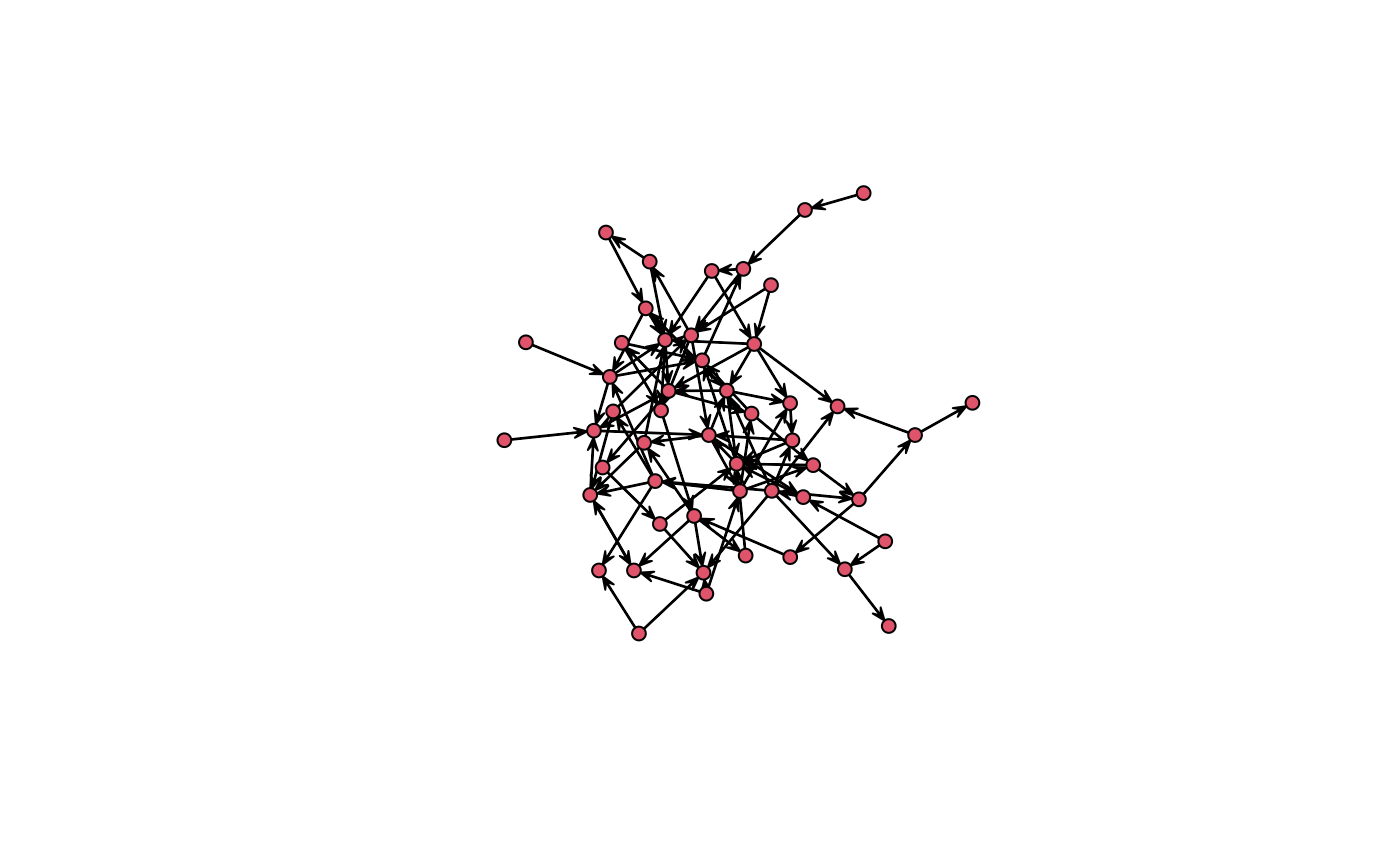
## and thus, networks after T=1 will be replaced with T-1.

Taking a look at it using sna

# Visualizing with 
gplot(as.matrix(net))

# Random diffusion with a fixed threshold of 1, simulating 5 time points
mydiffnet <- rdiffnet(
  seed.graph     = net,                    # The network we just created
  threshold.dist = 1,                      # Fixed threshold of 1
  t              = 5,                      # 5 time points
  rewire         = FALSE,                  # No rewire (defaults TRUE)
  exposure.args  = list(normalized=FALSE), # Exposure to be computed unnormalized 
                                           # so we use counts instead
  seed.nodes     = "random"                # Random set of initial adopters
  )

# Looking at the diffusion process
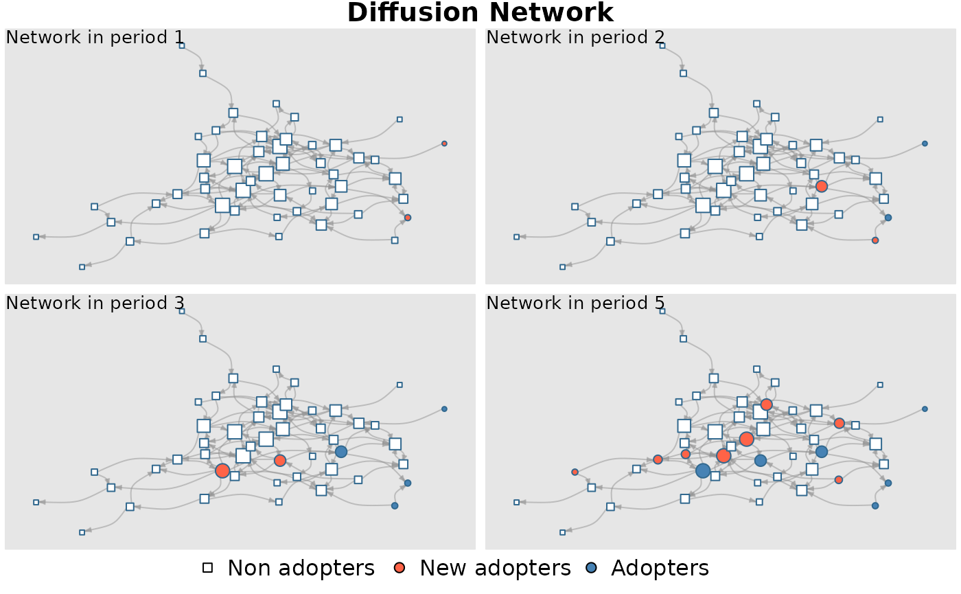
plot_diffnet(mydiffnet)

# Some summary stats
summary(mydiffnet)

## Diffusion network summary statistics
## Name     : A diffusion network
## Behavior : Random contagion
## -----------------------------------------------------------------------------
##  Period   Adopters   Cum Adopt. (%)   Hazard Rate   Density   Moran's I (sd)  
## -------- ---------- ---------------- ------------- --------- ---------------- 
##        1          2         2 (0.04)             -      0.04  0.00 (0.03)     
##        2          2         4 (0.08)          0.04      0.04  0.15 (0.03) *** 
##        3          2         6 (0.12)          0.04      0.04  0.10 (0.03) *** 
##        4          3         9 (0.18)          0.07      0.04  0.08 (0.03) *** 
##        5          5        14 (0.28)          0.12      0.04  0.07 (0.04) *** 
## -----------------------------------------------------------------------------
##  Left censoring  : 0.04 (2)
##  Right centoring : 0.72 (36)
##  # of nodes      : 50
## 
##  Moran's I was computed on contemporaneous autocorrelation using 1/geodesic
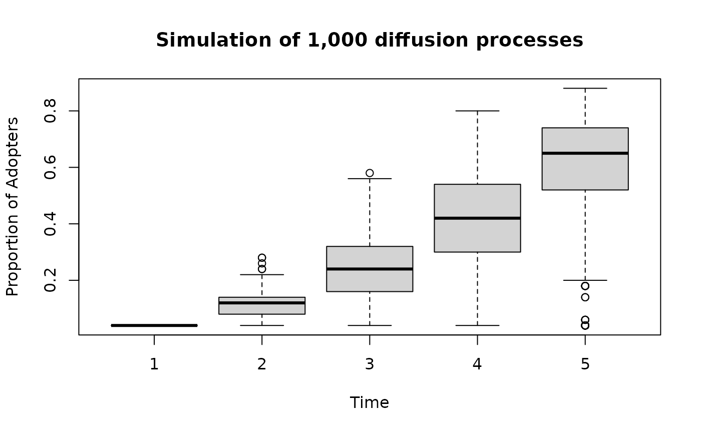
##  values. Significane levels  *** <= .01, ** <= .05, * <= .1.

We can actually go further and run multiple simulations instead so that we can get a confidence interval in the proportion of adopters

set.seed(871)
mydiffnet <- rdiffnet_multiple(
  statistic      = function(n) cumulative_adopt_count(n)["prop",],
  R              = 1000,
  stop.no.diff   = FALSE,                  # This option allows us to continue
                                           # The simulation process, even if there
                                           # is no adoption.
  seed.graph     = net,                    # The network we just created
  threshold.dist = 1,                      # Fixed threshold of 1
  t              = 5,                      # 5 time points
  rewire         = FALSE,                  # No rewire (defaults TRUE)
  exposure.args  = list(normalized=FALSE), # Exposure to be computed unnormalized 
                                           # so we use counts instead
  seed.nodes     = "random"                # Random set of initial adopters
  )

# Looking at the diffusion process
boxplot(
  t(mydiffnet),
  xlab = "Time",
  ylab = "Proportion of Adopters",
  main = "Simulation of 1,000 diffusion processes"
  )