Bass Model

Fits the Bass Diffusion model. In particular, fits an observed curve of proportions of adopters to \(F(t)\), the proportion of adopters at time \(t\), finding the corresponding coeficients \(p\), Innovation rate, and \(q\), imitation rate.

fitbass(dat, ...)

# S3 method for diffnet
fitbass(dat, ...)

# S3 method for default
fitbass(dat, ...)

# S3 method for diffnet_bass
plot(
  x,
  y = 1:length(x$m$lhs()),
  add = FALSE,
  pch = c(21, 24),
  main = "Bass Diffusion Model",
  ylab = "Proportion of adopters",
  xlab = "Time",
  type = c("b", "b"),
  lty = c(2, 1),
  col = c("black", "black"),
  bg = c("lightblue", "gray"),
  include.legend = TRUE,
  ...
)

bass_F(Time, p, q)

bass_dF(p, q, Time)

bass_f(Time, p, q)

Arguments

dat	Either a diffnet object, or a numeric vector. Observed cumulative proportion of adopters.
...	Further arguments passed to the method.
x	An object of class diffnet_bass.
y	Integer vector. Time (label).
add	Passed to matplot.
pch	Passed to matplot.
main	Passed to matplot.
ylab	Character scalar. Label of the y axis.
xlab	Character scalar. Label of the x axis.
type	Passed to matplot.
lty	Passed to matplot.
col	Passed to matplot.
bg	Passed to matplot.
include.legend	Logical scalar. When TRUE, draws a legend.
Time	Integer vector with values greater than 0. The \(t\) parameter.
p	Numeric scalar. Coefficient of innovation.
q	Numeric scalar. Coefficient of imitation.

Value

An object of class nls and diffnet_bass. For more details, see nls in the stats package.

Details

The function fits the bass model with parameters \([p, q]\) for values \(t = 1, 2, \dots, T\), in particular, it fits the following function:

$$ F(t) = \frac{1 - \exp{-(p+q)t}}{1 + \frac{q}{p}\exp{-(p+q)t}} $$

Which is implemented in the bass_F function. The proportion of adopters at time \(t\), \(f(t)\) is:

$$ f(t) = \left\{\begin{array}{ll} F(t), & t = 1 \\ F(t) - F(t-1), & t > 1 \end{array}\right. $$

and it's implemented in the bass_f function.

For testing purposes only, the gradient of \(F\) with respect to \(p\) and \(q\) is implemented in bass_dF.

The estimation is done using nls.

References

Bass's Basement Institute Institute. The Bass Model. (2010). Available at: http://www.bassbasement.org/BassModel/Default.aspx. (Accessed: 29th March 2017)

See also

Other statistics: classify_adopters(), cumulative_adopt_count(), dgr(), ego_variance(), exposure(), hazard_rate(), infection(), moran(), struct_equiv(), threshold(), vertex_covariate_dist()

Examples

# Fitting the model for the Brazilian Farmers Data --------------------------
data(brfarmersDiffNet)
ans <- fitbass(brfarmersDiffNet)

# All the methods that work for the -nls- object work here
ans
#> Nonlinear regression model
#>   model: dat ~ bass_F(Time, p, q)
#>    data: parent.frame()
#>        p        q 
#> 0.002279 0.336735 
#>  residual sum-of-squares: 0.05184
#> 
#> Number of iterations to convergence: 10 
#> Achieved convergence tolerance: 3.567e-06
summary(ans)
#> 
#> Formula: dat ~ bass_F(Time, p, q)
#> 
#> Parameters:
#>    Estimate Std. Error t value Pr(>|t|)    
#> p 0.0022787  0.0007245   3.145  0.00533 ** 
#> q 0.3367353  0.0268004  12.565 1.19e-10 ***
#> ---
#> Signif. codes:  0 ‘***’ 0.001 ‘**’ 0.01 ‘*’ 0.05 ‘.’ 0.1 ‘ ’ 1
#> 
#> Residual standard error: 0.05223 on 19 degrees of freedom
#> 
#> Number of iterations to convergence: 10 
#> Achieved convergence tolerance: 3.567e-06
#> 
coef(ans)
#>           p           q 
#> 0.002278742 0.336735345 
vcov(ans)
#>               p             q
#> p  5.249308e-07 -1.888583e-05
#> q -1.888583e-05  7.182629e-04

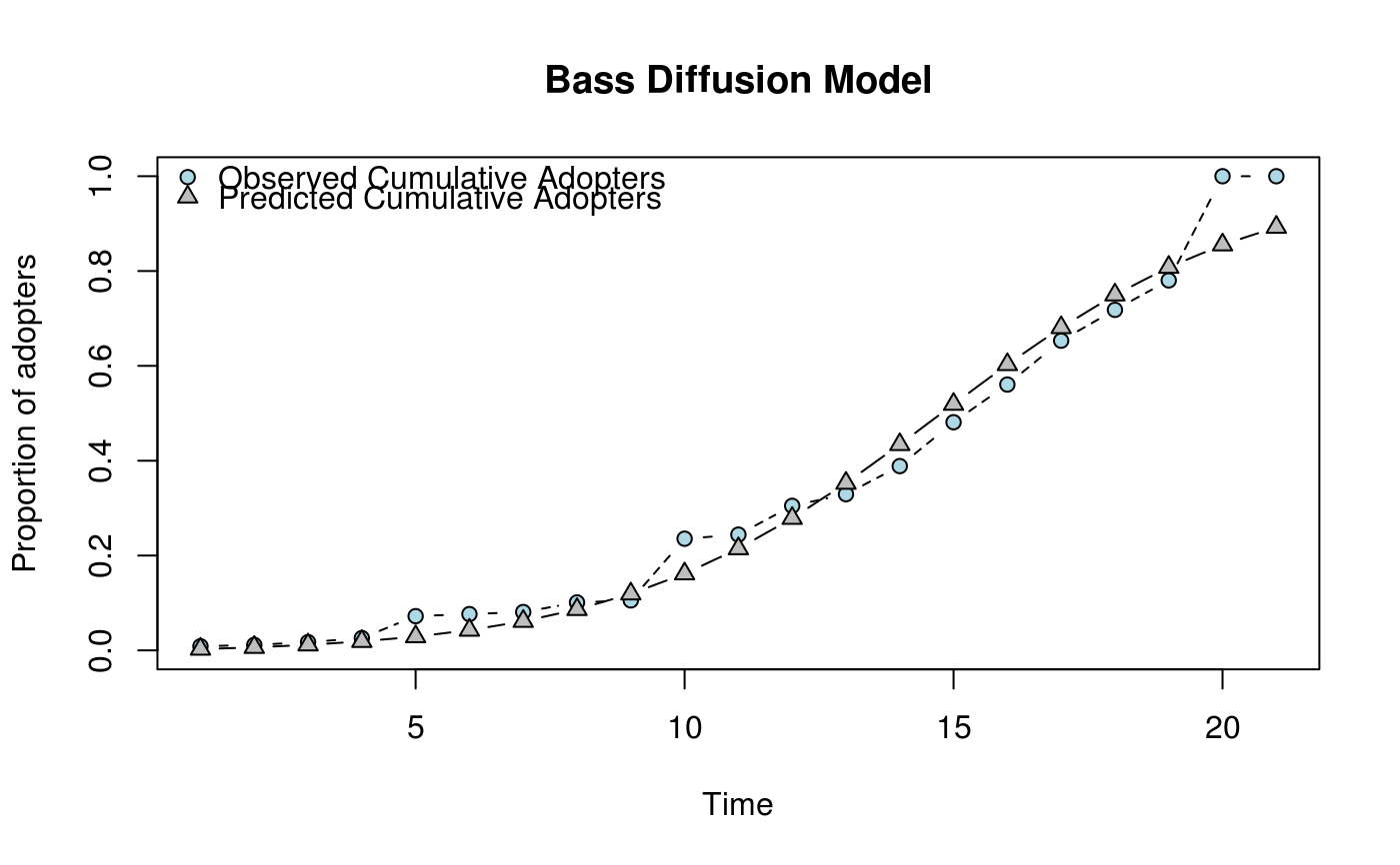
# And the plot method returns both, fitted and observed curve
plot(ans)