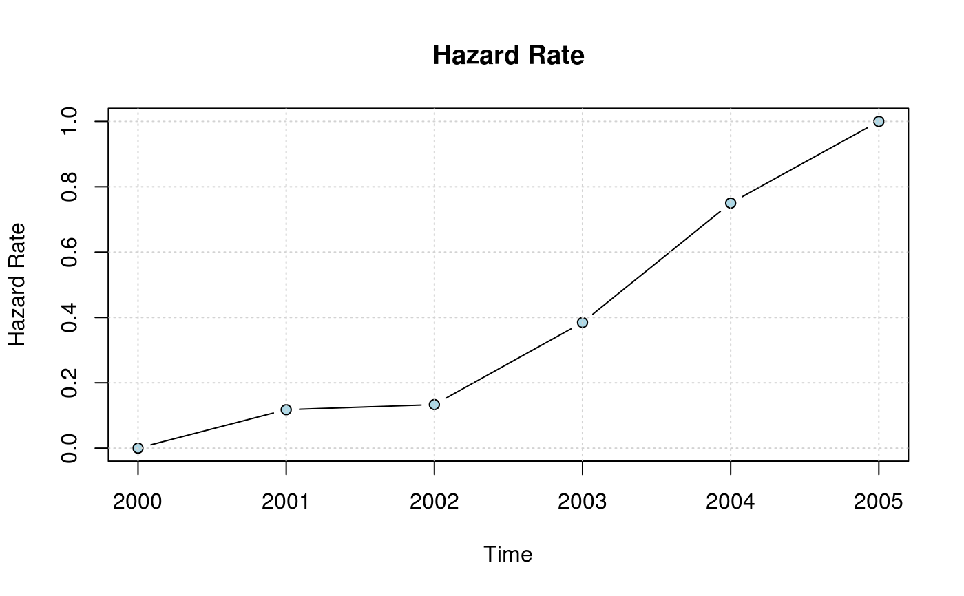
The hazard rate is the instantaneous probability of adoption at each time representing the likelihood members will adopt at that time (Allison 1984). The shape of the hazard rate indicates the pattern of new adopters over time. Rapid diffusion with convex cumulative adoption curves will have hazard functions that peak early and decay over time whereas slow concave cumulative adoption curves will have hazard functions that are low early and rise over time. Smooth hazard curves indicate constant adoption whereas those that oscillate indicate variability in adoption behavior over time.
Arguments
- obj
A \(n\times T\) matrix (Cumulative adoption matrix obtained from
toa_mat) or adiffnetobject.- no.plot
Logical scalar. When TRUE, suppress plotting (only returns hazard rates).
- include.grid
Logical scalar. When TRUE includes a grid on the plot.
- ...
further arguments to be passed to the method.
- x
An object of class
diffnet_hr.- y
ignored.
- main
Character scalar. Title of the plot
- xlab
Character scalar. x-axis label.
- ylab
Character scalar. y-axis label.
- type
Character scalar. See
par.- bg
Character scalar. Color of the points.
- pch
Integer scalar. See
par.- add
Logical scalar. When TRUE it adds the hazard rate to the current plot.
- ylim
Numeric vector. See
plot.
Value
A row vector of size \(T\) with hazard rates for \(t>1\) of class diffnet_hr.
The class of the object is only used by the S3 plot method.
Details
This function computes hazard rate, plots it and returns the hazard rate vector invisible (so is not printed on the console). For \(t>1\), hazard rate is calculated as
$$\frac{q_t - q_{t-1}}{n - q_{t-1}}$$
where \(q_i\) is the number of adopters in time \(t\), and \(n\) is the number of vertices in the graph.
In survival analysis, hazard rate is defined formally as
$$% \lambda(t)=\lim_{h\to +0}\frac{F(t+h)-F(t)}{h}\frac{1}{1-F(t)} % $$
Then, by approximating \(h=1\), we can rewrite the equation as
$$% \lambda(t)=\frac{F(t+1)-F(t)}{1-F(t)} % $$
Furthermore, we can estimate \(F(t)\), the probability of not having adopted the innovation in time \(t\), as the proportion of adopters in that time, this is \(F(t) \sim q_t/n\), so now we have
$$% \lambda(t)=\frac{q_{t+1}/n-q_t/n}{1-q_t/n} = \frac{q_{t+1} - q_t}{n - q_t} % $$
As showed above.
The plot_hazard function is an alias for the plot.diffnet_hr method.
References
Allison, P. (1984). Event history analysis regression for longitudinal event data. Beverly Hills: Sage Publications.
Wooldridge, J. M. (2010). Econometric Analysis of Cross Section and Panel Data (2nd ed.). Cambridge: MIT Press.
See also
Other statistics:
bass,
classify_adopters(),
cumulative_adopt_count(),
degree_adoption_diagnostic(),
dgr(),
ego_variance(),
exposure(),
infection(),
moran(),
struct_equiv(),
threshold(),
vertex_covariate_dist()
Other visualizations:
dgr(),
diffusionMap(),
drawColorKey(),
grid_distribution(),
plot_adopters(),
plot_diffnet(),
plot_diffnet2(),
plot_infectsuscep(),
plot_threshold(),
rescale_vertex_igraph()