Classify adopters accordingly to Time of Adoption and Threshold levels.
Source:R/stats.R
classify_adopters.RdAdopters are classified as in Valente (1995). In general, this is done depending on the distance in terms of standard deviations from the mean of Time of Adoption and Threshold.
classify_adopters(...)

classify(...)

# S3 method for class 'diffnet'
classify_adopters(graph, include_censored = FALSE, ...)

# Default S3 method
classify_adopters(
  graph,
  toa,
  t0 = NULL,
  t1 = NULL,
  expo = NULL,
  include_censored = FALSE,
  ...
)

# S3 method for class 'diffnet_adopters'
ftable(x, as.pcent = TRUE, digits = 2, ...)

# S3 method for class 'diffnet_adopters'
as.data.frame(x, row.names = NULL, optional = FALSE, ...)

# S3 method for class 'diffnet_adopters'
plot(x, y = NULL, ftable.args = list(), table.args = list(), ...)
Arguments
- ...
Further arguments passed to the method.
- graph
A dynamic graph.
- include_censored
Logical scalar, passed to
threshold.- toa
Integer vector of length \(n\) with times of adoption.
- t0
- t1
Integer scalar passed to
toa_mat.- expo
Numeric matrix of size \(n\times T\) with network exposures.
- x
A
diffnet_adoptersclass object.- as.pcent
Logical scalar. When
TRUEreturns a table with percentages instead.- digits
Integer scalar. Passed to
round.- row.names
Passed to
as.data.frame.- optional
Passed to
as.data.frame.- y
Ignored.
- ftable.args
List of arguments passed to
ftable.- table.args
List of arguments passed to
table.
Value
A list of class diffnet_adopters with the following elements:
- toa
A factor vector of length \(n\) with 4 levels: "Early Adopters", "Early Majority", "Late Majority", and "Laggards"
- thr
A factor vector of length \(n\) with 4 levels: "Very Low Thresh.", "Low Thresh.", "High Thresh.", and "Very High Thresh."
Details
Classifies (only) adopters according to time of adoption and threshold as described in Valente (1995). In particular, the categories are defined as follow:
For Time of Adoption, with toa as the vector of times of adoption:
Early Adopters:
toa[i] <= mean(toa) - sd(toa),Early Majority:
mean(toa) - sd(toa) < toa[i] <= mean(toa),Late Majority:
mean(toa) < toa[i] <= mean(toa) + sd(toa), andLaggards:
mean(toa) + sd(toa) < toa[i].
For Threshold levels, with thr as the vector of threshold levels:
Very Low Thresh.:
thr[i] <= mean(thr) - sd(thr),Low Thresh.:
mean(thr) - sd(thr) < thr[i] <= mean(thr),High Thresh.:
mean(thr) < thr[i] <= mean(thr) + sd(thr), andVery High. Thresh.:
mean(thr) + sd(thr) < thr[i].
By default threshold levels are not computed for left censored data. These
will have a NA value in the thr vector.
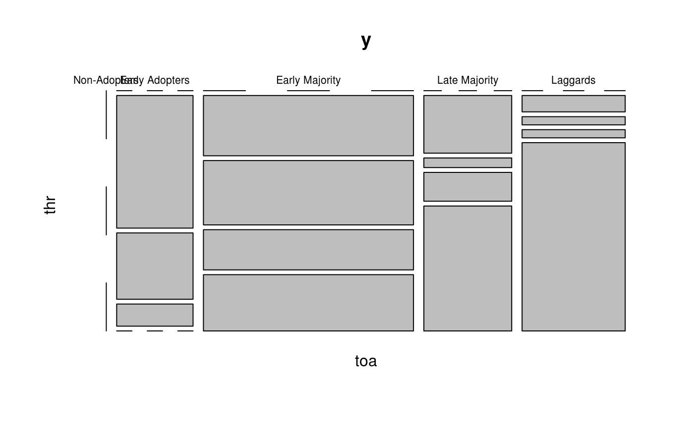
The plot method, plot.diffnet_adopters, is a wrapper for the
plot.table method. This generates a
mosaicplot plot.
References
Valente, T. W. (1995). "Network models of the diffusion of innovations" (2nd ed.). Cresskill N.J.: Hampton Press.
See also
Examples
# Classifying brfarmers -----------------------------------------------------

x <- brfarmersDiffNet
diffnet.toa(x)[x$toa==max(x$toa, na.rm = TRUE)] <- NA
out <- classify_adopters(x)

# This is one way
round(
with(out, ftable(toa, thr, dnn=c("Time of Adoption", "Threshold")))/
  nnodes(x[!is.na(x$toa)])*100, digits=2)
#>                  Threshold Non-Adopters Very Low Thresh. Low Thresh. High Thresh. Very High Thresh.
#> Time of Adoption
#> Non-Adopters                      28.15             0.00        0.00         0.00              0.00
#> Early Adopters                     0.00             7.96        3.70         0.74              1.11
#> Early Majority                     0.00             8.89       10.56         4.63              4.63
#> Late Majority                      0.00             6.30       10.19         8.70             16.30
#> Laggards                           0.00             1.48        1.11         2.22             11.48

# This is other
ftable(out)
#>                thr Non-Adopters Very Low Thresh. Low Thresh. High Thresh. Very High Thresh.
#> toa
#> Non-Adopters              21.97             0.00        0.00         0.00              0.00
#> Early Adopters             0.00             6.21        2.89         0.58              0.87
#> Early Majority             0.00             6.94        8.24         3.61              3.61
#> Late Majority              0.00             4.91        7.95         6.79             12.72
#> Laggards                   0.00             1.16        0.87         1.73              8.96

# Can be coerced into a data.frame, e.g. ------------------------------------
 str(classify(brfarmersDiffNet))
#> List of 3
#>  $ toa    : Factor w/ 5 levels "Non-Adopters",..: 4 5 4 3 3 4 4 3 5 4 ...
#>  $ thr    : Factor w/ 5 levels "Non-Adopters",..: 4 4 4 3 3 4 4 3 4 4 ...
#>  $ cutoffs:List of 2
#>   ..$ toa: num [1:3] 1955 1960 1965
#>   ..$ thr: num [1:3] 0.206 0.614 1.021
#>  - attr(*, "class")= chr "diffnet_adopters"
 ans <- cbind(
 as.data.frame(classify(brfarmersDiffNet)), brfarmersDiffNet$toa
 )
 head(ans)
#>                 toa          thr brfarmersDiffNet$toa
#> 1001  Late Majority High Thresh.                 1961
#> 1002       Laggards High Thresh.                 1965
#> 1004  Late Majority High Thresh.                 1963
#> 1005 Early Majority  Low Thresh.                 1957
#> 1007 Early Majority  Low Thresh.                 1959
#> 1009  Late Majority High Thresh.                 1960

# Creating a mosaic plot with the medical innovations -----------------------
x <- classify(medInnovationsDiffNet)
plot(x)