Visualization

Visualization methods

netdiffuseR offers several methods to visualize network diffusion dynamics. Here we will focus on three of them: plot_adopters(), plot_threshold(), and plot_diffnet().

You can see the Reference Manual on CRAN, or the Appendix from this lecture, to see the full list of methods available in the package.

Creating a diffusion network with survey_to_diffnet()

We can select a specific village and visualize its diffusion dynamics. As we did in the previous section, we will use the kfamily dataset, which contains data on Korean Family Planning, and we will focus on village #21:

data(kfamily)

# Subset the kfamily dataset for village 21
kfamily_21 <- subset(kfamily, village == 21)

# Convert the subsetted data to a diffnet object
kfamily_diffnet_21 <- survey_to_diffnet(
  dat      = kfamily_21,
  idvar    = "id",
  netvars  = c(
    # Neighbors talk to about FP
    "net11", "net12", "net13", "net14", "net15", 
    # Closest neighbor most frequently met
    "net21", "net22", "net23", "net24", "net25", 
    # Advice on FP sought from 
    "net31", "net32", "net33", "net34", "net35"), 
  toavar   = "toa",
  groupvar = "village"
)

We can visualize adopters and cumulative adopters:

plot_adopters(kfamily_diffnet_21)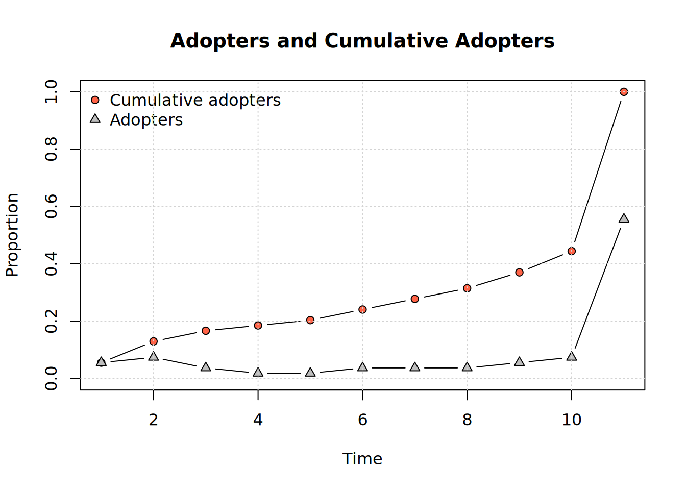

or draw a graph where the x-axis coordinates are given by time of adoption, and the y-axis by the threshold level:

plot_threshold(kfamily_diffnet_21)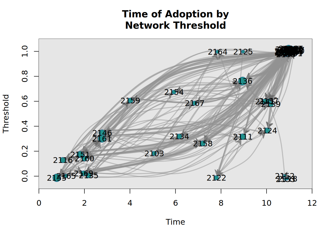

or create a colored network plot showing the diffusion status of the graph through time (one network plot for each time period):

plot_diffnet(kfamily_diffnet_21)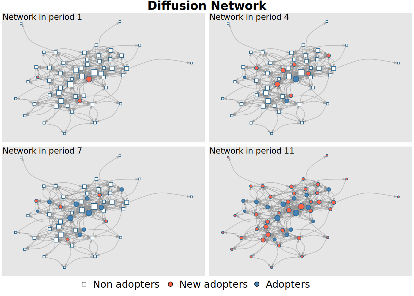

Problems

1. Using the diffnet object in intro.rda, use the function plot_threshold specifying shapes and colors according to the variables ItrustMyFriends and Age. Do you see any pattern? (solution script and solution plot)

Appendix

Creating a diffusion network with rdiffnet()

Another example using the rdiffnet function to generate random diffusion networks. This example creates a small-world network with 400 nodes and 6 time steps, where the connections are rewired based on a threshold distance of 1/4. The seed.graph is set to “small-world” and the seed.nodes to “central”, which means that the initial nodes are chosen from the center of the network.

set.seed(12315)
diffnet_1 <- rdiffnet(
  n = 400, t = 6,
  rgraph.args    = list(k=6, p=.3),
  seed.graph     = "small-world",
  seed.nodes     = "central",
  rewire         = FALSE,
  threshold.dist = 1/4
  )
diffnet_1

# Dynamic network of class -diffnet-
#  Name               : A diffusion network
#  Behavior           : Random contagion
#  # of nodes         : 400 (1, 2, 3, 4, 5, 6, 7, 8, ...)
#  # of time periods  : 6 (1 - 6)
#  Type               : directed
#  Num of behaviors   : 1
#  Final prevalence   : 0.95
#  Static attributes  : real_threshold (1)
#  Dynamic attributes : -

Diffusion networks can visualized using many methods included in the package. Here are some of them:

plot(diffnet_1)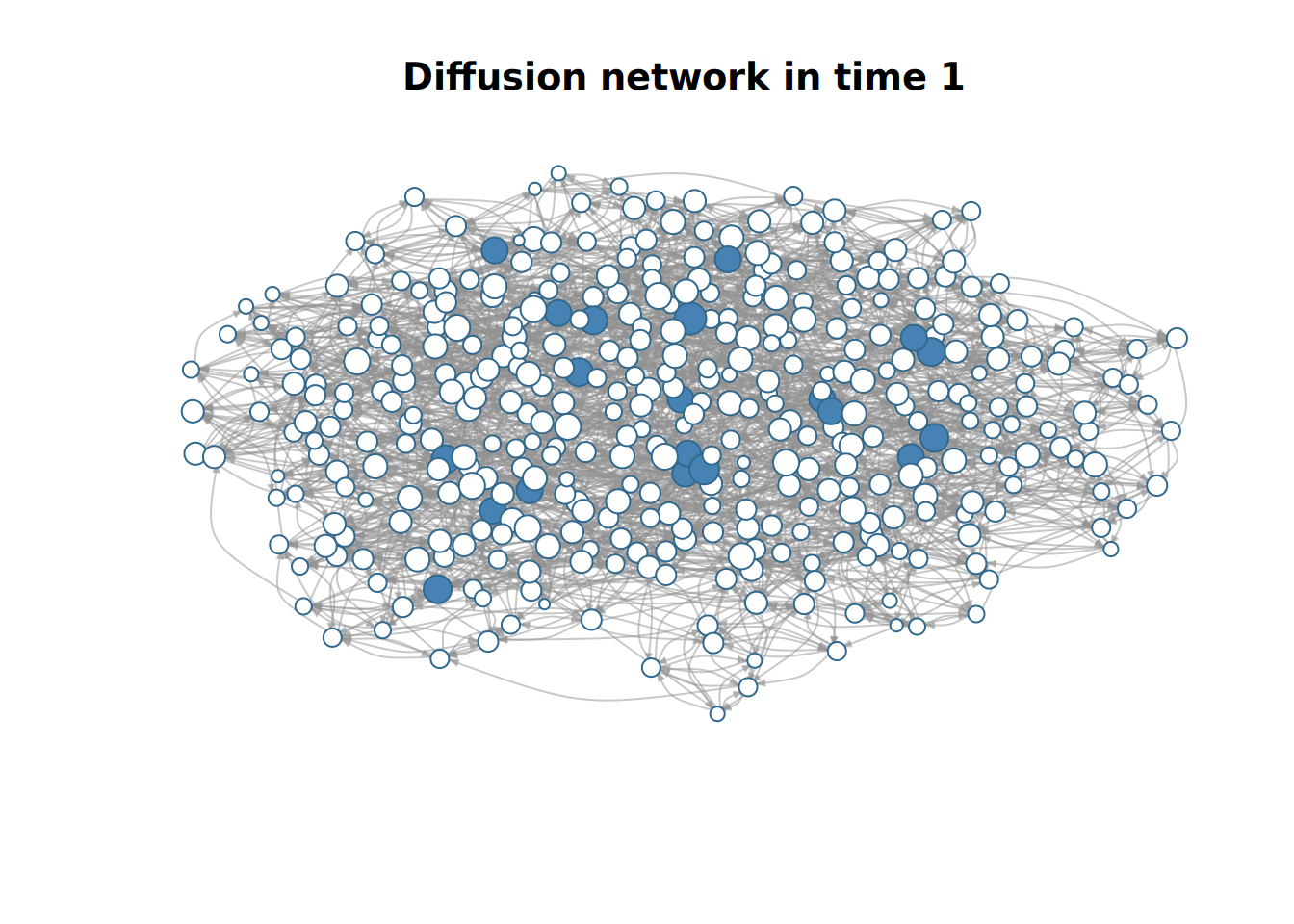

plot_diffnet(diffnet_1)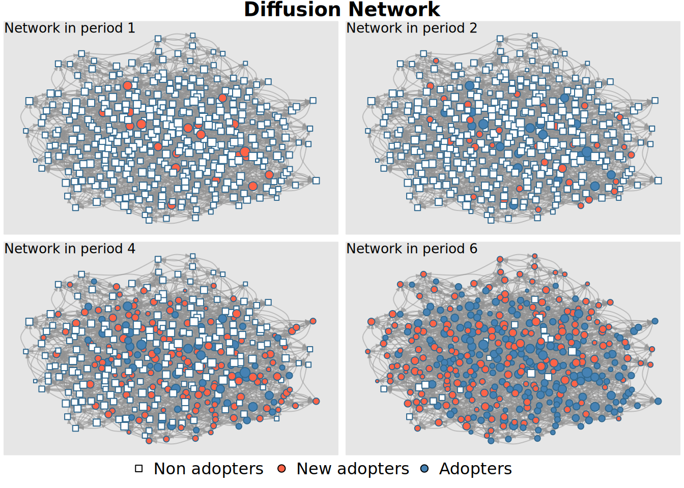

plot_diffnet2(diffnet_1)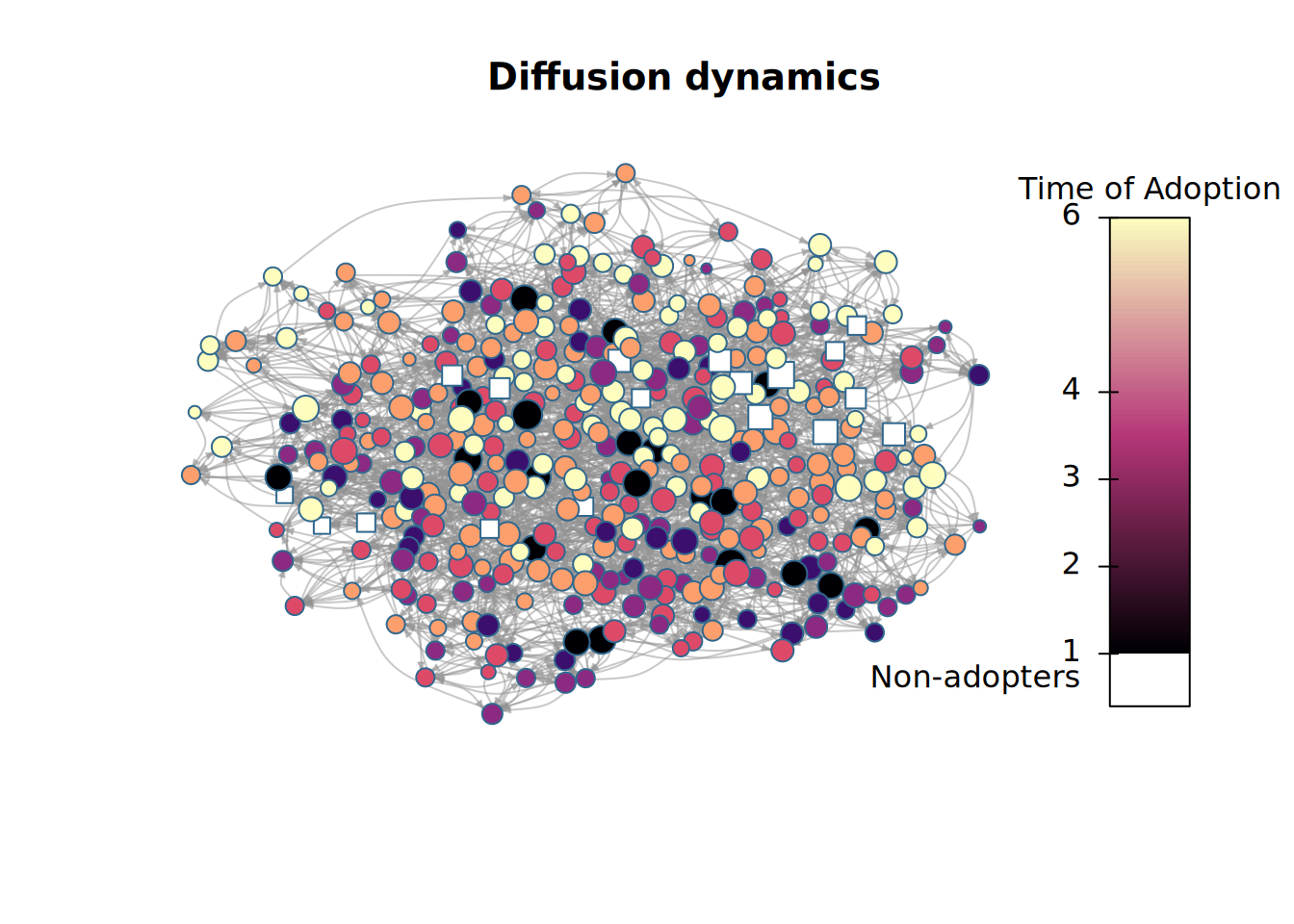

plot_adopters(diffnet_1)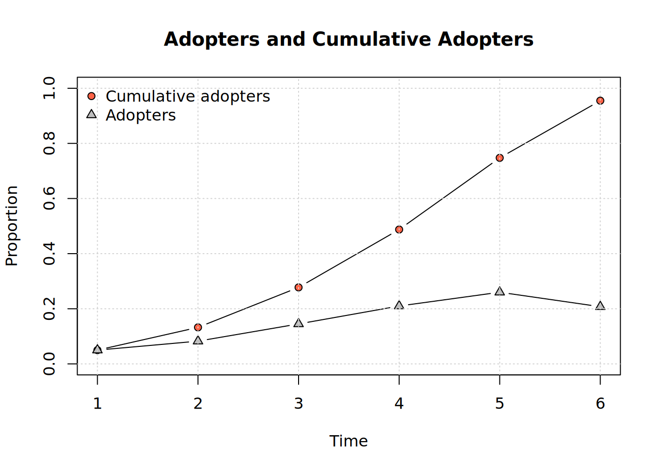

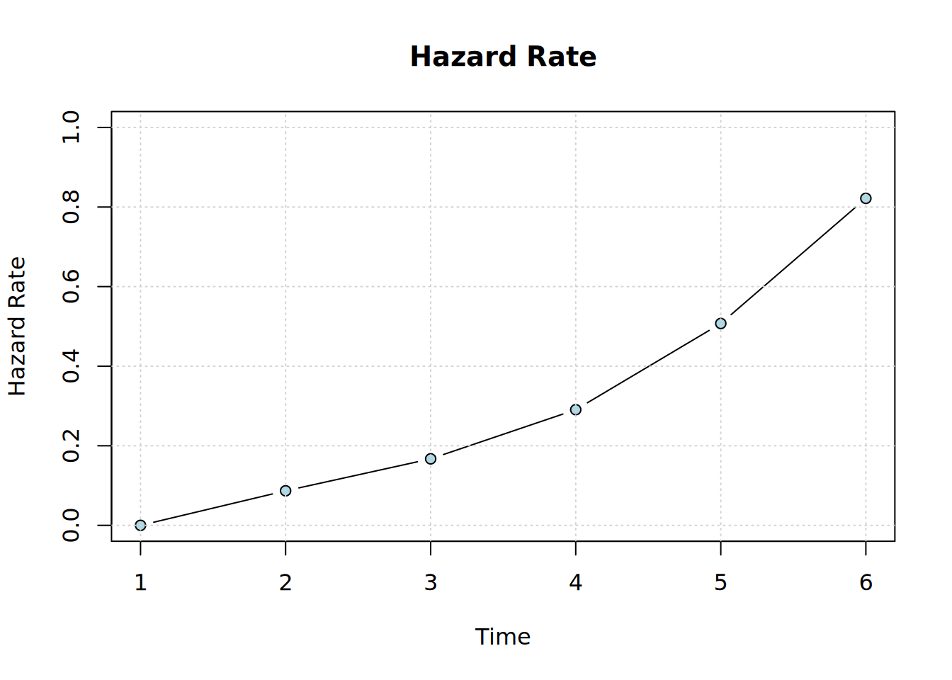
plot_threshold(diffnet_1)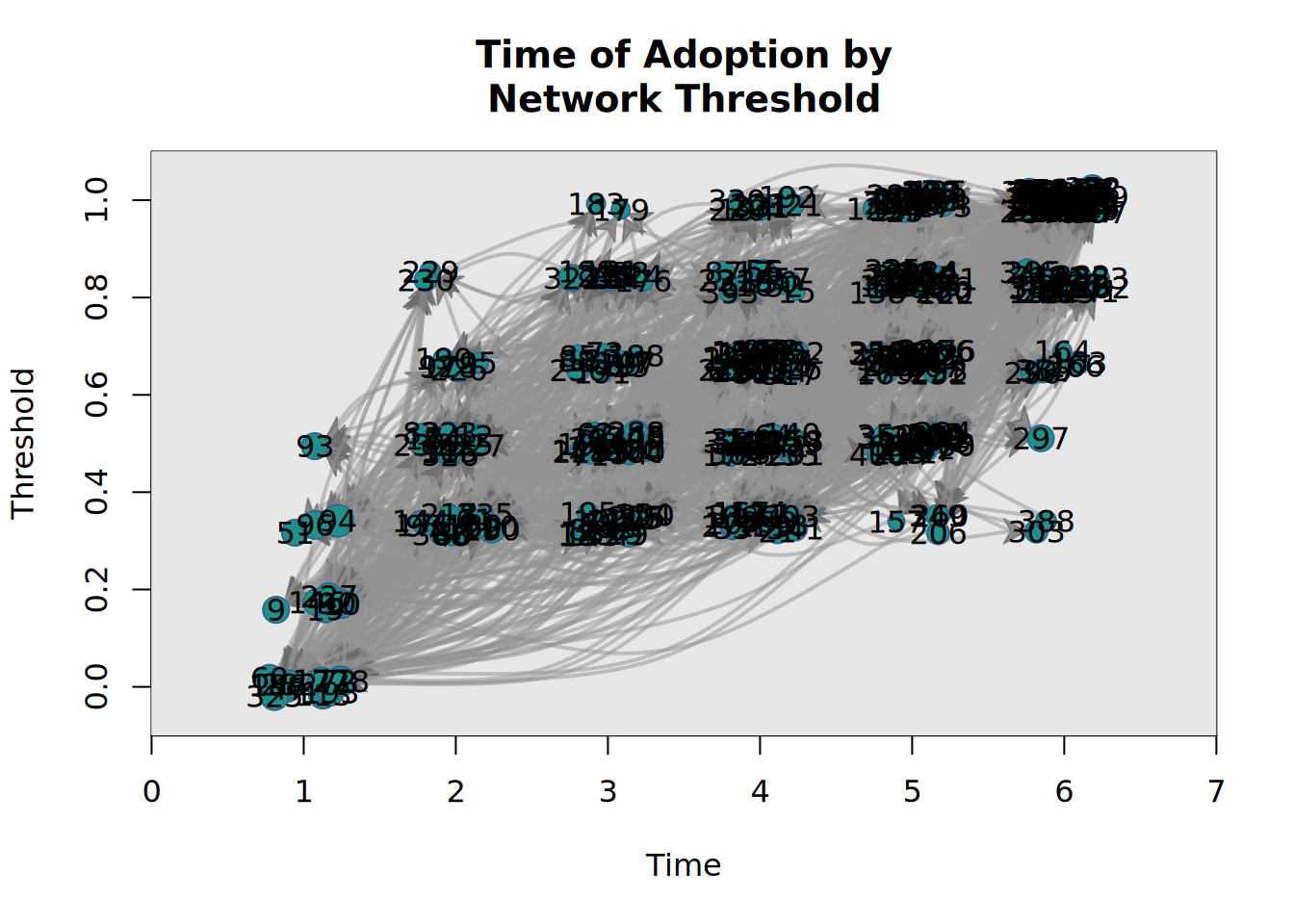

plot_infectsuscep(diffnet_1, K=2)

# Warning in plot_infectsuscep.list(graph$graph, graph$toa, t0, normalize, : When
# applying logscale some observations are missing.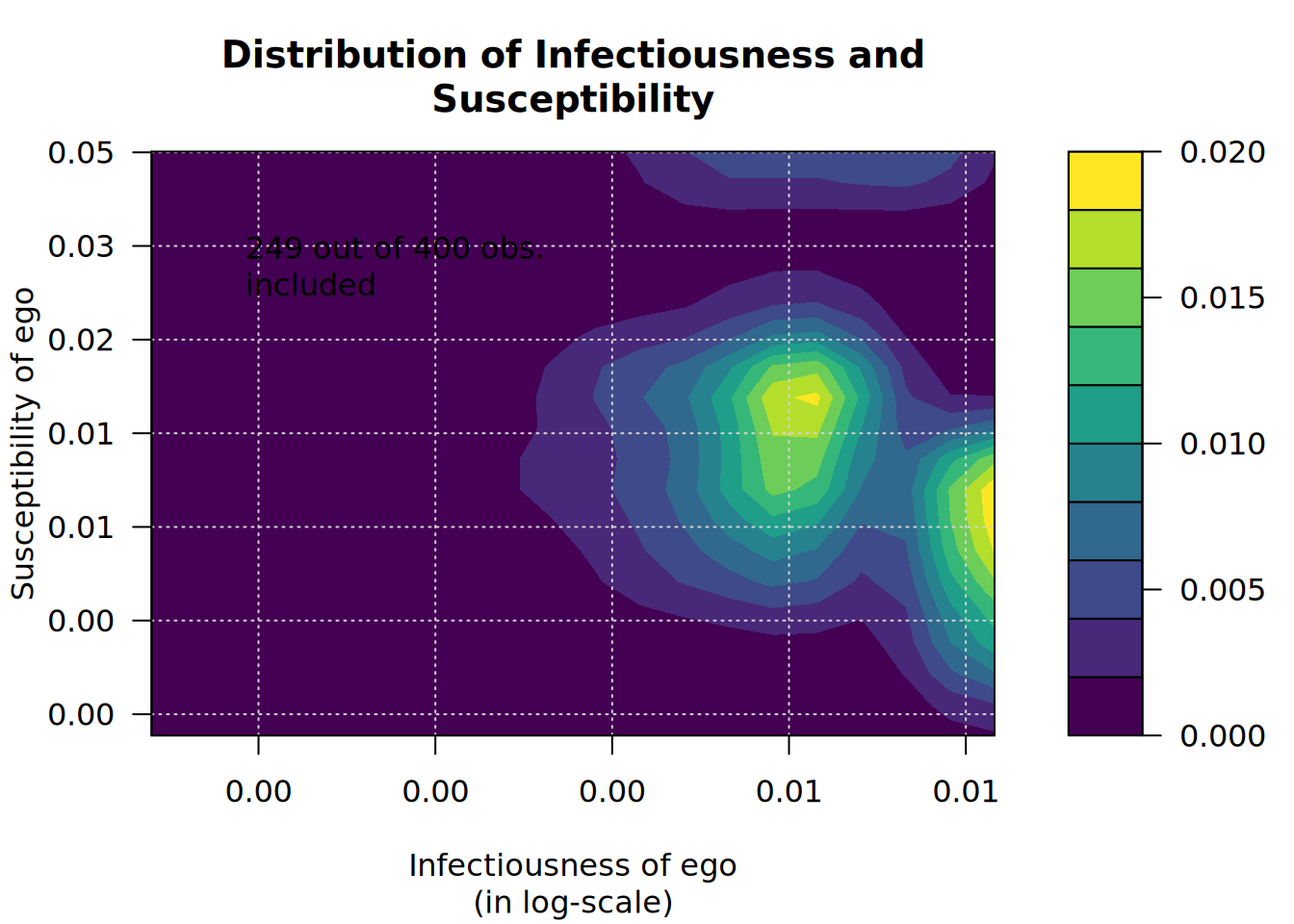

plot_hazard(diffnet_1)