Simulation of diffusion networks: multi- and dis- adoption

Multiadoption and Disadoption

netdiffuseR supports simulating multi- and dis-adoption diffusion processes.

Next, let’s use an empirical network:

data(kfamily)
kfamily_21 <- subset(kfamily, village == 21)

kfamily_diffnet_21 <- survey_to_diffnet(
  dat      = kfamily_21,
  idvar    = "id",
  netvars  = c(
    "net11", "net12", "net13", "net14", "net15", 
    "net21", "net22", "net23", "net24", "net25", 
    "net31", "net32", "net33", "net34", "net35"), 
  toavar   = "toa",
  groupvar = "village"
)

plot_diffnet(kfamily_diffnet_21, slices = c(1, 9))

Multiadoption simulations

To study a multi-adoption process, you can pass a list as the seed.p.adopt parameter.

Here is a simple example with two behaviors, passing a diffnet object as input, which already contains the seed graph and time points:

set.seed(1231)
diffnet_1 <- rdiffnet(
  seed.graph     = kfamily_diffnet_21,
  seed.p.adopt   = list(0.15, 0.1),                            # <-- two behaviors
  threshold.dist = runif(nvertices(kfamily_diffnet_21), .3,.5)
)

diffnet_1

# Dynamic network of class -diffnet-
#  Name               : A diffusion network
#  Behavior           : Random contagion_1, Random contagion_2
#  # of nodes         : 54 (1, 2, 3, 4, 5, 6, 7, 8, ...)
#  # of time periods  : 11 (1 - 11)
#  Type               : directed
#  Num of behaviors   : 2
#  Prevalence         : 0.96, 0.69
#  Static attributes  : real_threshold.1, real_threshold.2 (2)
#  Dynamic attributes : -

Multiadoption visualization

We can use the split_behaviors function to split a diffnet object into a list of diffnet objects.

Tip

Until now, the multi-adoption module simulates behaviors independently, so the code above is equivalent to simulating the same behavior twice. Models with interdependent behaviors are supported via the disadopt parameter.

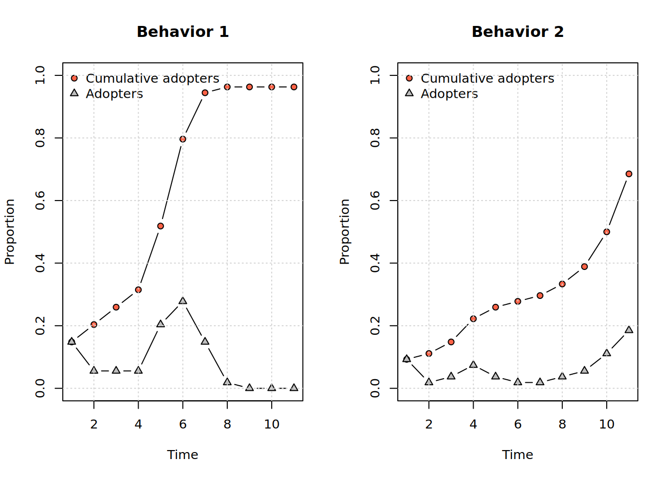
Then, we can use the plot_adopters (or any single-adoption function) to visualize the diffusion process for each behavior:

diffnets_1 <- split_behaviors(diffnet_1)

op <- par(mfrow=c(1,2), cex = .8)
plot_adopters(diffnets_1[[1]], main = "Behavior 1")
plot_adopters(diffnets_1[[2]], main = "Behavior 2")

par(op)

Disadoption

The rdiffnet function includes the disadopt parameter to add a disadoption function, that:

1. Receives three arguments: expo, cumadopt, and time.

   1. expo is the exposure array with three dimensions: # of nodes $\times$ # of time points $\times$ # of behaviors.
   2. cumadopt is the cumulative adoption array, with the same dimensions as expo. So, if cumadopt[i, t, q] = 1, then i is an adopter of behavior q at time t.
   3. time is the current time point in the simulation.

2. Must return a list with one element per behavior: the $q$-th element is a vector with the nodes that disadopt behavior $q$.

3. If no node disadopts a given behavior, return an empty vector integer() for that element.

disadoption_function <- function(expo, cumadopt, time) {
  
  # Some calculations..
  
  return(list( disadopters_1, disadopters_2, integer() ))
}

Example of disadoption parameter

We can build a disadoption function that restricts nodes from adopting more than one behavior at a time:

$$\text{Disadopt_1}_{it} = \left\{\begin{array}{l}Yes,\quad\text{if behavior 2 has adopted}\\\text{No},\quad\text{otherwise.}\end{array}\right.$$

The following code shows how to build such a function:

second_only <- function(expo, cumadopt, time) {

 # Identifying double adopters
 ids <- which(rowSums(cumadopt[, time, ]) == 2)

 # If there are no double adopters, return an empty list
 if (length(ids) == 0)
   return(list(integer(), integer()))

 # Otherwise, make them disadopt the first behavior
 return(list(ids, integer()))
}

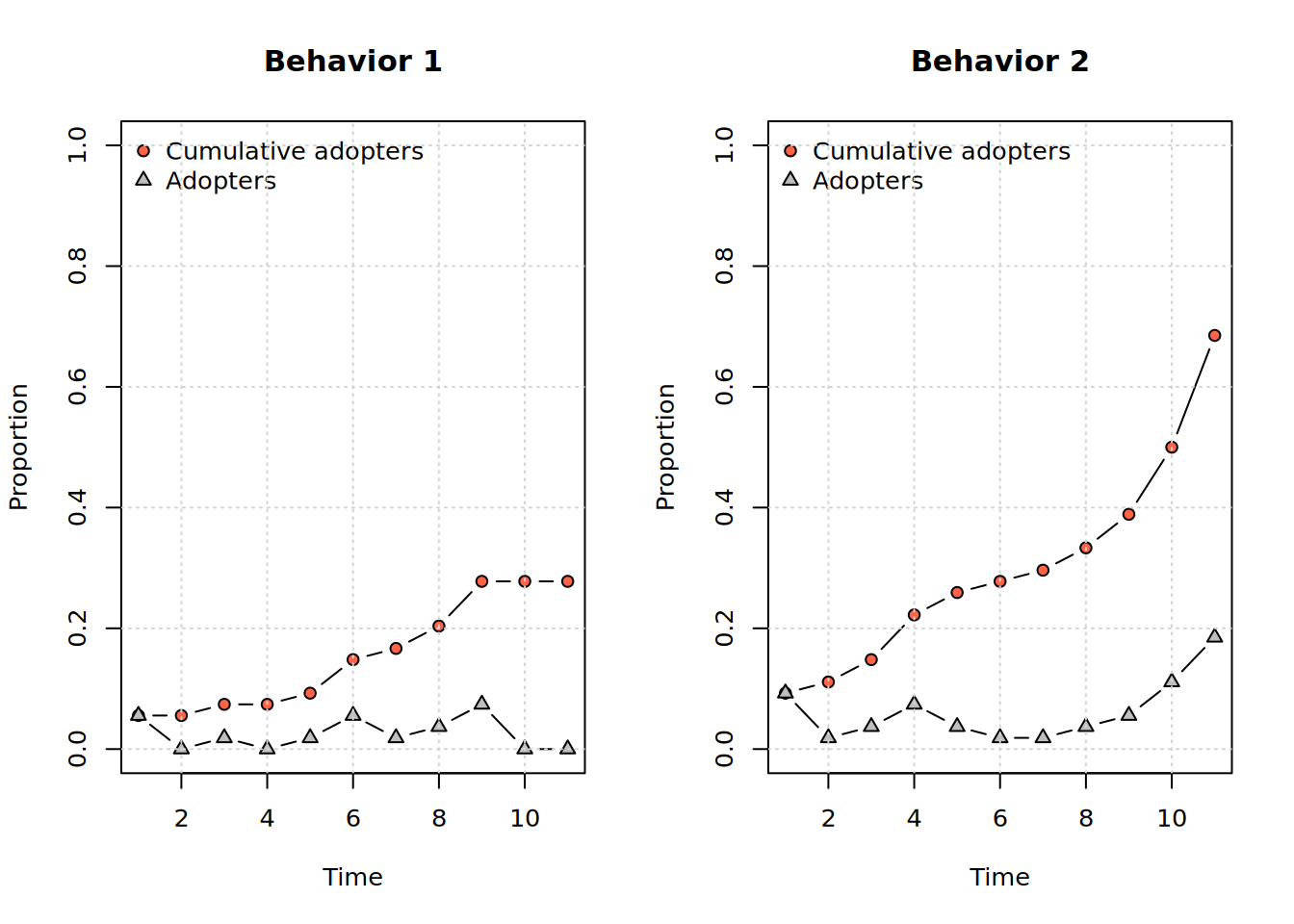
Let’s simulate a diffusion process with the disadoption function second_only:

set.seed(1231)

diffnet_2 <- rdiffnet(
  seed.graph     = kfamily_diffnet_21,
  seed.p.adopt   = list(0.15, 0.10),
  threshold.dist = runif(nvertices(kfamily_diffnet_21), .3,.5),
  disadopt       = second_only                                 # <-- disadop function
)

diffnets_2 <- split_behaviors(diffnet_2)

op <- par(mfrow=c(1,2), cex = .8)
plot_adopters(diffnets_2[[1]], main = "Behavior 1")
plot_adopters(diffnets_2[[2]], main = "Behavior 2")

par(op)

Exercises

1. Using the template for a disadoption function,

  disadoption_function <- function(expo, cumadopt, time) {
    
    # 1) set number of behaviors
    # 2) iterate through the behaviors
    # 3) identify adopters at time t - 1
    # 4) select 10% of adopters to disadopt
    # 5) if there are no disadopters, return(list(integer(), integer()))
    
  }

create a disadoption function that randomly selects 10% of the adopters at time t - 1 for $q$ behaviors. (solution file)

2. Create a disadoption function that makes younger individuals disadopt sooner. You can use the kfamily dataset. (solution file)

3. Using the template for a disadoption function, create a disadoption function that simulates a fashion that dies incrementally over time. You can try this for one or more fads. (solution file)

Appendix

Other examples with multiadoption

To study a multi-adoption process, you can pass a list as the seed.p.adopt parameter.

Here is a simple example with two behaviors and synthetic data:

set.seed(123)

n <- 200
t <- 10

graph <- rgraph_ws(n, t, p=.3)  # Watts-Strogatz model

diffnet_3 <- rdiffnet(
 seed.graph = graph,
 t = t,
 seed.p.adopt = list(0.1, 0.15)
 )

diffnet_3

# Dynamic network of class -diffnet-
#  Name               : A diffusion network
#  Behavior           : Random contagion_1, Random contagion_2
#  # of nodes         : 200 (1, 2, 3, 4, 5, 6, 7, 8, ...)
#  # of time periods  : 10 (1 - 10)
#  Type               : directed
#  Num of behaviors   : 2
#  Prevalence         : 0.83, 0.92
#  Static attributes  : real_threshold.1, real_threshold.2 (2)
#  Dynamic attributes : -

The “Num of behaviors” entry now shows 2, the “Behavior” entry also shows two behaviors, "Random contagion \_1, Random contagion\_2", and finally, the “Prevalence” entry also shows two numbers: 0.29, 0.97.

We can specify different parameters for each behavior:

set.seed(1231)

diffnet_4 <- rdiffnet(
 seed.graph = graph,
 t = t,
 seed.p.adopt = list(0.1, 0.15),
 threshold.dist = list(
   runif(n, .3, .5),
   runif(n, .2, .4)
 ),
 seed.nodes = list("central", "random"),
 behavior   = list("tobacco", "alcohol")
)

diffnet_4

# Dynamic network of class -diffnet-
#  Name               : A diffusion network
#  Behavior           : tobacco, alcohol
#  # of nodes         : 200 (1, 2, 3, 4, 5, 6, 7, 8, ...)
#  # of time periods  : 10 (1 - 10)
#  Type               : directed
#  Num of behaviors   : 2
#  Prevalence         : 0.91, 1.00
#  Static attributes  : real_threshold.1, real_threshold.2 (2)
#  Dynamic attributes : -

See the rdiffnet documentation for more details on the parameters for multiadoption.