Network thresholds (Valente, 1995; 1996), \(\tau\), are defined as the required proportion or number of neighbors that leads you to adopt a particular behavior, \(a=1\).
where \(E_i\) is i’s exposure to the innovation and \(\mathbf{X}\) is the adjacency matrix (the network). Here is a review of the concepts we will be using:
Exposure \(E_i\) : Proportion/number of neighbors that has adopted an innovation at each point in time.
Threshold \(\tau\) : The proportion/number of your neighbors who had adopted at or one time period before ego (the focal individual) adopted.
Infectiousness: How much \(i\)’s adoption affects her alters.
Susceptibility: How much \(i\)’s alters’ adoption affects her.
Structural equivalence: How similar are \(i\) and \(j\) in terms of position in the network.
Simulating diffusion networks
We can simulate a diffusion using the rdiffnet function included in the package. The simulation algorithm is as follows:
Pick the graph you give in the input, or a complex baseline graph is created if required (\(N\) nodes),
The set of \(t\) networks is created (if required),
Set of initial adopters and threshold distribution (one \(\tau_i\) per node) are established,
Simulation starts at \(t=2\), assigning adopters based on exposures and thresholds:
For each \(i \in N\), if its exposure at \(t-1\) is greater than its threshold, then adopts. Otherwise continue without change.
next \(i\)
Let’s construct a first diffusion network with
500 nodes,
Spanning 10 time periods,
The seeds (initial adopters) will be selected randomly,
Seeds will be a 5% of the network,
The graph will be small-world,
With a probability of rewire \(p=0.2\),
Threshold levels will be uniformly distributed between [0.3, 0.7]
# Setting the seed for the RNGset.seed(1213)# Generating a random diffusion networkdiffnet_behavior <-rdiffnet(n =500, # 1.t =10, # 2.seed.nodes ="random", # 3.seed.p.adopt = .05, # 4.seed.graph ="small-world", # 5.rgraph.args =list(p=.2), # 6.threshold.dist =function(x) runif(1, .3, .7) # 7. )diffnet_behavior
# Dynamic network of class -diffnet-
#  Name               : A diffusion network
#  Behavior           : Random contagion
#  # of nodes         : 500 (1, 2, 3, 4, 5, 6, 7, 8, ...)
#  # of time periods  : 10 (1 - 10)
#  Type               : directed
#  Num of behaviors   : 1
#  Final prevalence   : 0.52
#  Static attributes  : real_threshold (1)
#  Dynamic attributes : -
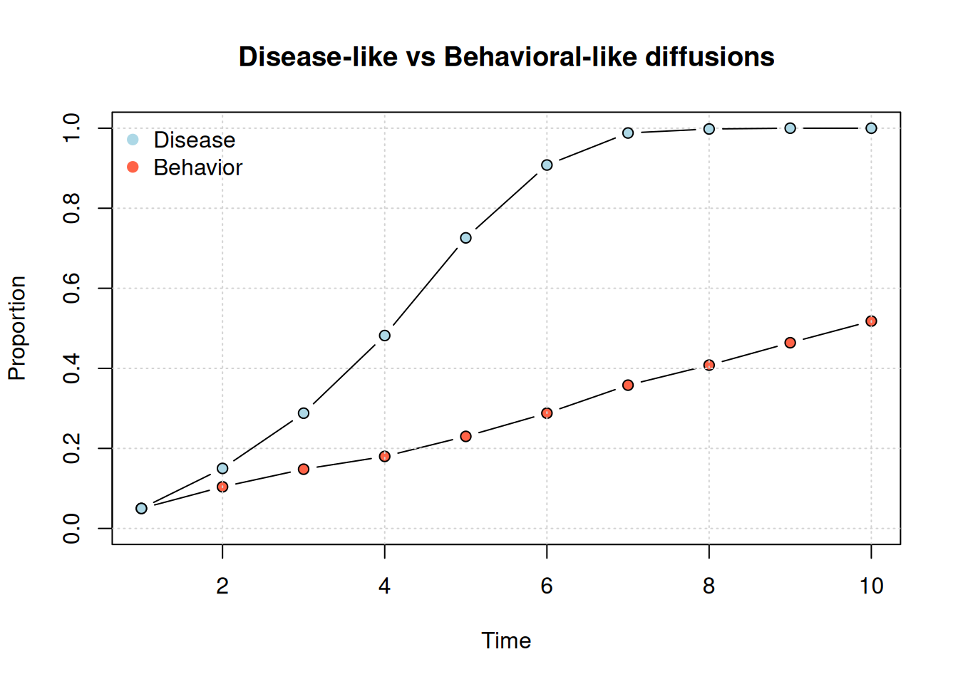
Simple vs Threshold diffusion
In disease-like diffusions, a single adopting neighbor is enough to adopt (absolute threshold \(= 1\)). In behavioral-like diffusions, or threshold diffusion, there should be more sources of influence (e.g., 30%).
plot_adopters(diffnet_behavior, what ="cumadopt", include.legend =FALSE,main ="Disease-like vs Behavioral-like diffusions")plot_adopters(diffnet_disease, bg="lightblue", add=TRUE, what ="cumadopt")legend("topleft",legend =c("Disease", "Behavior"),col =c("lightblue", "tomato"),bty ="n", pch=19 )
Problems
The default degree of our Watts-Strogatz network is k = 2. Re-run the disease-like and the behavioral-like diffusions on a denser, more clustered network using k = 5, keeping everything else fixed. Which one speeds up, which one slows down, and why? (solution script and solution plot)
Using the Korean family village 21, compare which strategy setting the seed nodes maximizes the diffusion. Use rdiffnet_multiple to run 500 simulations for each strategy. The strategies are:
Given the following types of networks: Small-world, Scale-free, Bernoulli, what set of \(n\) initiators (central, marginal, or random) maximizes diffusion? (solution script and solution plot)
Appendix
rdiffnet_multiple in a nutshell
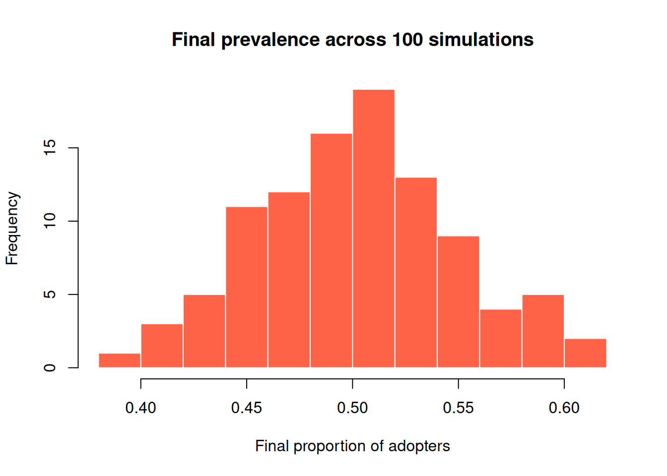
A single diffusion is just one realization of a random process. To learn how a diffusion behaves on average, we repeat it many times. rdiffnet_multiple() does exactly that.
Let’s reuse diffnet_behavior as the seed graph and, across 100 simulations, keep the final prevalence:
set.seed(123)final_prevalence <-rdiffnet_multiple(R =100L, # number of simulationsstatistic =function(x) sum(!is.na(x$toa))/500,seed.graph = diffnet_behavior,seed.nodes ="random",seed.p.adopt = .05,threshold.dist =runif(500, .3, .7))hist(final_prevalence, col ="tomato", border ="white",xlab ="Final proportion of adopters",main ="Final prevalence across 100 simulations")
Example by changing threshold (rdiffnet_multiple)
The following block of code runs multiple diffnet simulations.
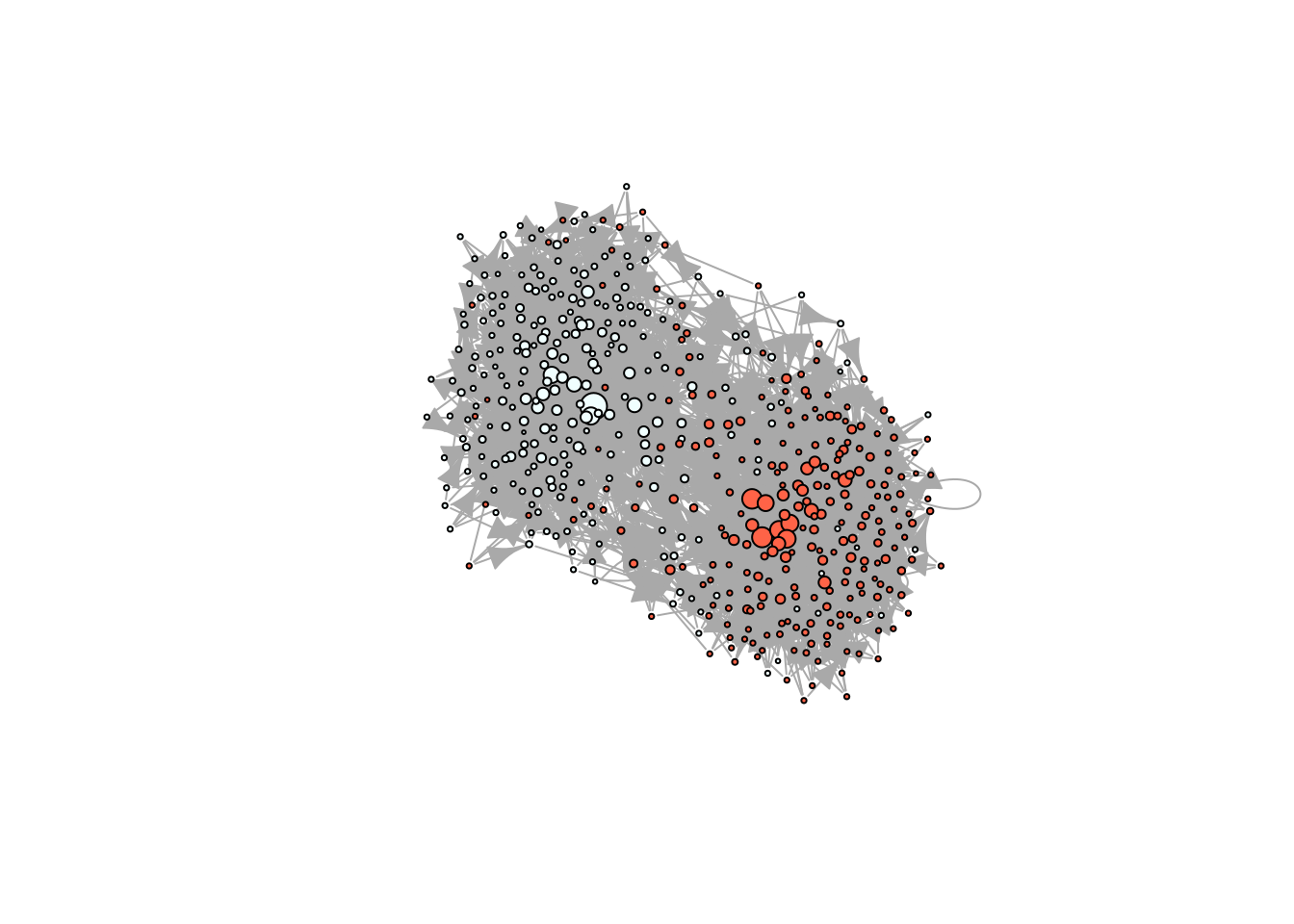
Before we proceed, we will generate a scale-free homophilic network using rgraph_ba:
# Simulating a scale-free homophilic networkset.seed(1231)X <-rep(c(1,1,1,1,1,0,0,0,0,0), 50)net <-rgraph_ba(t =499, m=4, eta = X)# Taking a look in igraphig <- igraph::graph_from_adjacency_matrix(net)plot(ig, vertex.color =c("azure", "tomato")[X+1], vertex.label =NA,vertex.size =sqrt(dgr(net)))
Besides the usual parameters passed to rdiffnet, the rdiffnet_multiple function requires:
R (number of repetitions/simulations), and
statistic (a function that returns the statistic of interest).
Optionally, the user may choose to specify the number of clusters to run it in parallel (multiple CPUs):
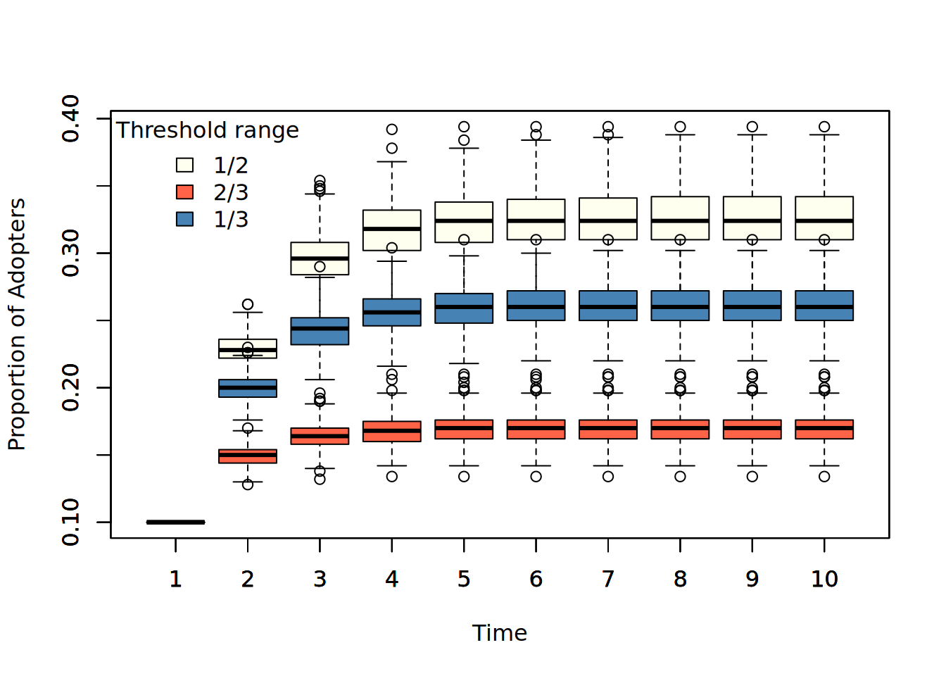
nsim <-500Lans_1and2 <-rdiffnet_multiple(# Num of simR = nsim,# Statisticstatistic =function(d) cumulative_adopt_count(d)["prop",], seed.graph = net,t =10,threshold.dist =sample(1:2, 500L, TRUE),seed.nodes ="random",seed.p.adopt = .1,rewire =FALSE,exposure.args =list(outgoing=FALSE, normalized=FALSE),# Running on 4 coresncpus =4L ) |>t()ans_2and3 <-rdiffnet_multiple(# Num of simR = nsim,# Statisticstatistic =function(d) cumulative_adopt_count(d)["prop",], seed.graph = net,t =10,threshold.dist =sample(2:3, 500, TRUE),seed.nodes ="random",seed.p.adopt = .1,rewire =FALSE,exposure.args =list(outgoing=FALSE, normalized=FALSE),# Running on 4 coresncpus =4L ) |>t()ans_1and3 <-rdiffnet_multiple(# Num of simR = nsim,# Statisticstatistic =function(d) cumulative_adopt_count(d)["prop",], seed.graph = net,t =10,threshold.dist =sample(1:3, 500, TRUE),seed.nodes ="random",seed.p.adopt = .1,rewire =FALSE,exposure.args =list(outgoing=FALSE, normalized=FALSE),# Running on 4 coresncpus =4L ) |>t()
By simulating 1000 times each diffusion, we can see the final prevalence is a function of threshold levels.