# Constructing diffusion network from village #21
kfamily_21 <- subset(kfamily, village == 21)

kfamily_diffnet_21 <- survey_to_diffnet(
  dat      = kfamily_21,
  idvar    = "id",
  netvars  = c(
    "net11", "net12", "net13", "net14", "net15",
    "net21", "net22", "net23", "net24", "net25",
    "net31", "net32", "net33", "net34", "net35"),
  toavar   = "toa",
  groupvar = "village"
)Statistical inference
Moran’s I
Moran’s I tests for spatial autocorrelation.
netdiffuseR implements the test in
moran, which is suited for sparse matrices.We can use Moran’s I as a first look to whether there is something happening: let that be influence or homophily.
Let’s see how to compute Moran’s I in netdiffuseR from a
diffnetobject:
Using geodesics
One approach is to use the geodesic (shortes path length) matrix to account for indirect influence.
In the case of sparse matrices, and furthermore, in the presence of structural holes it is more convenient to calculate the distance matrix taking this into account.
netdiffuseR has a function to do so, the
approx_geodesicfunction which, using graph powers, computes the shortest path up tonsteps. What happens under the hood is:# For each time point we compute the geodesic distances matrix W <- approx_geodesic(kfamily_diffnet_21$graph[[1]]) # We get the element-wise inverse W@x <- 1/W@x # And then compute moran moran(kfamily_diffnet_21$cumadopt[,1], W)# $observed # [1] -0.02559265 # # $expected # [1] -0.01886792 # # $sd # [1] 0.009505065 # # $p.value # [1] 0.4792627 # # attr(,"class") # [1] "diffnet_moran"
Using summary()
The
summary.diffnetmethod already runs Moran’s for you.summary(kfamily_diffnet_21)# Diffusion network summary statistics # Name : Diffusion Network # Behavior : Unknown # ----------------------------------------------------------------------------- # Period Adopters Cum Adopt. (%) Hazard Rate Density Moran's I (sd) # -------- ---------- ---------------- ------------- --------- ---------------- # 1 3 3 (0.06) - 0.10 -0.03 (0.01) # 2 4 7 (0.13) 0.08 0.10 -0.03 (0.01) # 3 2 9 (0.17) 0.04 0.10 -0.02 (0.01) # 4 1 10 (0.19) 0.02 0.10 -0.01 (0.01) # 5 1 11 (0.20) 0.02 0.10 -0.02 (0.01) # 6 2 13 (0.24) 0.05 0.10 -0.01 (0.01) # 7 2 15 (0.28) 0.05 0.10 -0.01 (0.01) # 8 2 17 (0.31) 0.05 0.10 -0.01 (0.01) # 9 3 20 (0.37) 0.08 0.10 -0.00 (0.01) * # 10 4 24 (0.44) 0.12 0.10 -0.00 (0.01) # 11 30 54 (1.00) 1.00 0.10 - # ----------------------------------------------------------------------------- # Left censoring : 0.06 (3) # Right centoring : 0.00 (0) # # of nodes : 54 # # Moran's I was computed on contemporaneous autocorrelation using 1/geodesic # values. Significane levels *** <= .01, ** <= .05, * <= .1.
Regression analysis
In regression analysis we want to see if exposure, once we control for other covariates, had any effect on the adoption of a behavior.
In general, the big problem here is when we have a latent variable that co-determines both network and behavior. Unless we can control for such variable, regression analysis will be generically biased.
If you can claim that either such variable doesn’t exists or you actually can control for it, then we have two options:
- lagged exposure models, or
- contemporaneous exposure models.
We will focus on the former.
Lagged exposure models
These models typically include the following structure:
\[ y_t = f(G_{t-1}, y_{t-1}, X_i) + \varepsilon, \]
Where the variable of interest \(y_t\) depends on:
- The previous state \(y_{t-1}\)
- The time-lagged adjacency matrix \(G_{t-1}\)
- Covariates \(X_i\)
For adoption scenarios, the model becomes:
\[ y_{it} = \left\{ \begin{array}{ll} 1 & \mbox{if}\quad \rho\sum_{j\neq i}\frac{G_{ijt-1}y_{it-1}}{\sum_{j\neq i}G_{ijt-1}} + X_{it}\beta > 0\\ 0 & \mbox{otherwise} \end{array} \right. \]
In netdiffuseR is as easy as doing the following:
# Adding 'cohesion' exposure
kfamily_diffnet_21[["exposure"]] <- exposure(kfamily_diffnet_21)

# Adding 'structructure equivalence' exposure
kfamily_diffnet_21[["exposure_se"]] <-  exposure(kfamily_diffnet_21,
                                                alt.graph="se",
                                                groupvar="village",
                                                valued=TRUE)

# Adding 'adoption'
kfamily_diffnet_21[["adoption"]] <- kfamily_diffnet_21$cumadopt

# pregs -> total pregnancie
# media12 -> Poster exposure to FP
model_1 <- diffreg(kfamily_diffnet_21 ~ exposure + exposure_se + media12 + sons + pregs + factor(per), type = "probit")

summary(model_1)
# # Call: # glm(formula = Adopt ~ exposure + exposure_se + media12 + sons + # pregs + factor(per), family = binomial(link = "probit"), # data = dat, subset = ifelse(is.na(toa), TRUE, toa >= per)) # # Coefficients: # Estimate Std. Error z value Pr(>|z|) # (Intercept) -2.18644 0.43386 -5.040 4.67e-07 *** # exposure 1.04034 0.54686 1.902 0.0571 . # exposure_se -2.94671 2.84852 -1.034 0.3009 # media12 -0.04793 0.15001 -0.319 0.7494 # sons 0.27766 0.10881 2.552 0.0107 * # pregs 0.04780 0.06008 0.796 0.4263 # factor(per)3 -0.35045 0.44722 -0.784 0.4333 # factor(per)4 -0.76292 0.54812 -1.392 0.1640 # factor(per)5 -0.72566 0.54987 -1.320 0.1869 # factor(per)6 -0.39806 0.49841 -0.799 0.4245 # factor(per)7 -0.22731 0.50078 -0.454 0.6499 # factor(per)8 -0.28374 0.54577 -0.520 0.6031 # factor(per)9 0.04869 0.55535 0.088 0.9301 # factor(per)10 0.39819 0.59764 0.666 0.5052 # factor(per)11 10.51465 250.12917 0.042 0.9665 # --- # Signif. codes: 0 '***' 0.001 '**' 0.01 '*' 0.05 '.' 0.1 ' ' 1 # # (Dispersion parameter for binomial family taken to be 1) # # Null deviance: 308.24 on 410 degrees of freedom # Residual deviance: 138.09 on 396 degrees of freedom # (54 observations deleted due to missingness) # AIC: 168.09 # # Number of Fisher Scoring iterations: 17This is equivalent to use
glmwithkfamily_diffnet_21as data frame.See the Appendix for an example of how to generate a synthetic dataset and run a regression model with it.
Problems
Using the dataset stats.rda:
Compute Moran’s I as the function
summary.diffnetdoes. For this you’ll need to use the functiontoa_mat(which calculates the cumulative adoption matrix), andapprox_geodesic(which computes the geodesic matrix). (see?summary.diffnetfor more details).Read the data as diffnet object, and fit the following logit model \(adopt = Exposure*\gamma + Measure*\beta + \varepsilon\). What happens if you exclude the time fixed effects?
Appendix
Lagged exposure models (synthetic)
# fakedata
set.seed(121)

W   <- rgraph_ws(1e3, 8, .2)
X   <- cbind(var1 = rnorm(1e3))
toa <- sample(c(NA,1:5), 1e3, TRUE)

dn  <- new_diffnet(W, toa=toa, vertex.static.attrs = X)

# Computing exposure and adoption for regression
dn[["cohesive_expo"]] <- cbind(NA, exposure(dn)[,-nslices(dn)])
dn[["adopt"]]         <- dn$cumadopt

# Running the model with `diffreg`
ans <- diffreg(dn ~ exposure + var1 + factor(per), type = "probit")
summary(ans)
#
# Call:
# glm(formula = Adopt ~ exposure + var1 + factor(per), family = binomial(link = "probit"),
# data = dat, subset = ifelse(is.na(toa), TRUE, toa >= per))
#
# Coefficients:
# Estimate Std. Error z value Pr(>|z|)
# (Intercept) -0.92777 0.05840 -15.888 < 2e-16 ***
# exposure 0.23839 0.17514 1.361 0.173452
# var1 -0.04623 0.02704 -1.710 0.087334 .
# factor(per)3 0.29313 0.07715 3.799 0.000145 ***
# factor(per)4 0.33902 0.09897 3.425 0.000614 ***
# factor(per)5 0.59851 0.12193 4.909 9.18e-07 ***
# ---
# Signif. codes: 0 '***' 0.001 '**' 0.01 '*' 0.05 '.' 0.1 ' ' 1
#
# (Dispersion parameter for binomial family taken to be 1)
#
# Null deviance: 2745.1 on 2317 degrees of freedom
# Residual deviance: 2663.5 on 2312 degrees of freedom
# (1000 observations deleted due to missingness)
# AIC: 2675.5
#
# Number of Fisher Scoring iterations: 4To do the same with glm, we need to do more work:
# Generating the data and running the model
dat <- as.data.frame(dn)
ans <- glm(adopt ~ cohesive_expo + var1 + factor(per),
           data = dat,
           family = binomial(link="probit"),
           subset = is.na(toa) | (per <= toa))
summary(ans)
#
# Call:
# glm(formula = adopt ~ cohesive_expo + var1 + factor(per), family = binomial(link = "probit"),
# data = dat, subset = is.na(toa) | (per <= toa))
#
# Coefficients:
# Estimate Std. Error z value Pr(>|z|)
# (Intercept) -0.92777 0.05840 -15.888 < 2e-16 ***
# cohesive_expo 0.23839 0.17514 1.361 0.173452
# var1 -0.04623 0.02704 -1.710 0.087334 .
# factor(per)3 0.29313 0.07715 3.799 0.000145 ***
# factor(per)4 0.33902 0.09897 3.425 0.000614 ***
# factor(per)5 0.59851 0.12193 4.909 9.18e-07 ***
# ---
# Signif. codes: 0 '***' 0.001 '**' 0.01 '*' 0.05 '.' 0.1 ' ' 1
#
# (Dispersion parameter for binomial family taken to be 1)
#
# Null deviance: 2745.1 on 2317 degrees of freedom
# Residual deviance: 2663.5 on 2312 degrees of freedom
# (1000 observations deleted due to missingness)
# AIC: 2675.5
#
# Number of Fisher Scoring iterations: 4Structural dependence and permutation tests
- A novel statistical method (work-in-progress) that allows conducting inference.
- Included in the package, tests whether a particular network statistic actually depends on network structure
- Suitable to be applied to network thresholds (you can’t use thresholds in regression-like models!)
Idea
Let \(\mathcal{G} = (V,E)\) be a graph, \(\gamma\) a vertex attribute, and \(\beta = f(\gamma,\mathcal{G})\), then
\[\gamma \perp \mathcal{G} \implies \mathbb{E}\left[\beta(\gamma,\mathcal{G})|\mathcal{G}\right] = \mathbb{E}\left[\beta(\gamma,\mathcal{G})\right]\]
This is, if for example time of adoption is independent on the structure of the network, then the average threshold level will be independent from the network structure as well.
Another way of looking at this is that the test will allow us to see how probable is to have this combination of network structure and network threshold (if it is uncommon then we say that the diffusion model is highly likely)
Example Not random TOA
- To use this test, netdiffuseR has the
struct_testfunction. - Basically it simulates networks with the same density and computes a particular statistic every time, generating an EDF (Empirical Distribution Function) under the Null hyphothesis (p-values).
# Simulating network
set.seed(1123)
net <- rdiffnet(n=500, t=10, seed.graph = "small-world")

# Running the test
test <- struct_test(
  graph     = net,
  statistic = function(x) mean(threshold(x), na.rm = TRUE),
  R         = 1e3,
  ncpus=4, parallel="multicore"
  )

# See the output
test
#
# Structure dependence test
# # Simulations : 1,000
# # nodes : 500
# # of time periods : 10
# --------------------------------------------------------------------------------
# H0: E[beta(Y,G)|G] - E[beta(Y,G)] = 0 (no structure dependency)
# observed expected p.val
# 0.5513 0.2516 0.0000hist(test)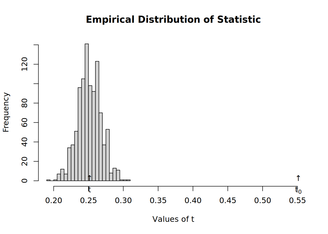
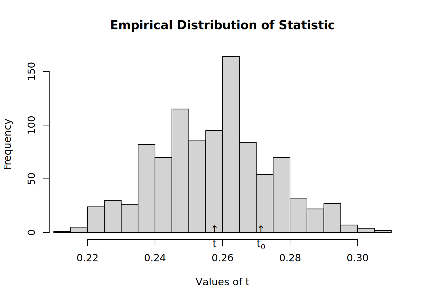
- Now we shuffle toas, so that is random
# Resetting TOAs (now will be completely random)
diffnet.toa(net) <- sample(diffnet.toa(net), nnodes(net), TRUE)

# Running the test
test <- struct_test(
  graph     = net,
  statistic = function(x) mean(threshold(x), na.rm = TRUE),
  R         = 1e3,
  ncpus=4, parallel="multicore"
  )

# See the output
test
#
# Structure dependence test
# # Simulations : 1,000
# # nodes : 500
# # of time periods : 10
# --------------------------------------------------------------------------------
# H0: E[beta(Y,G)|G] - E[beta(Y,G)] = 0 (no structure dependency)
# observed expected p.val
# 0.2714 0.2591 0.4220hist(test)