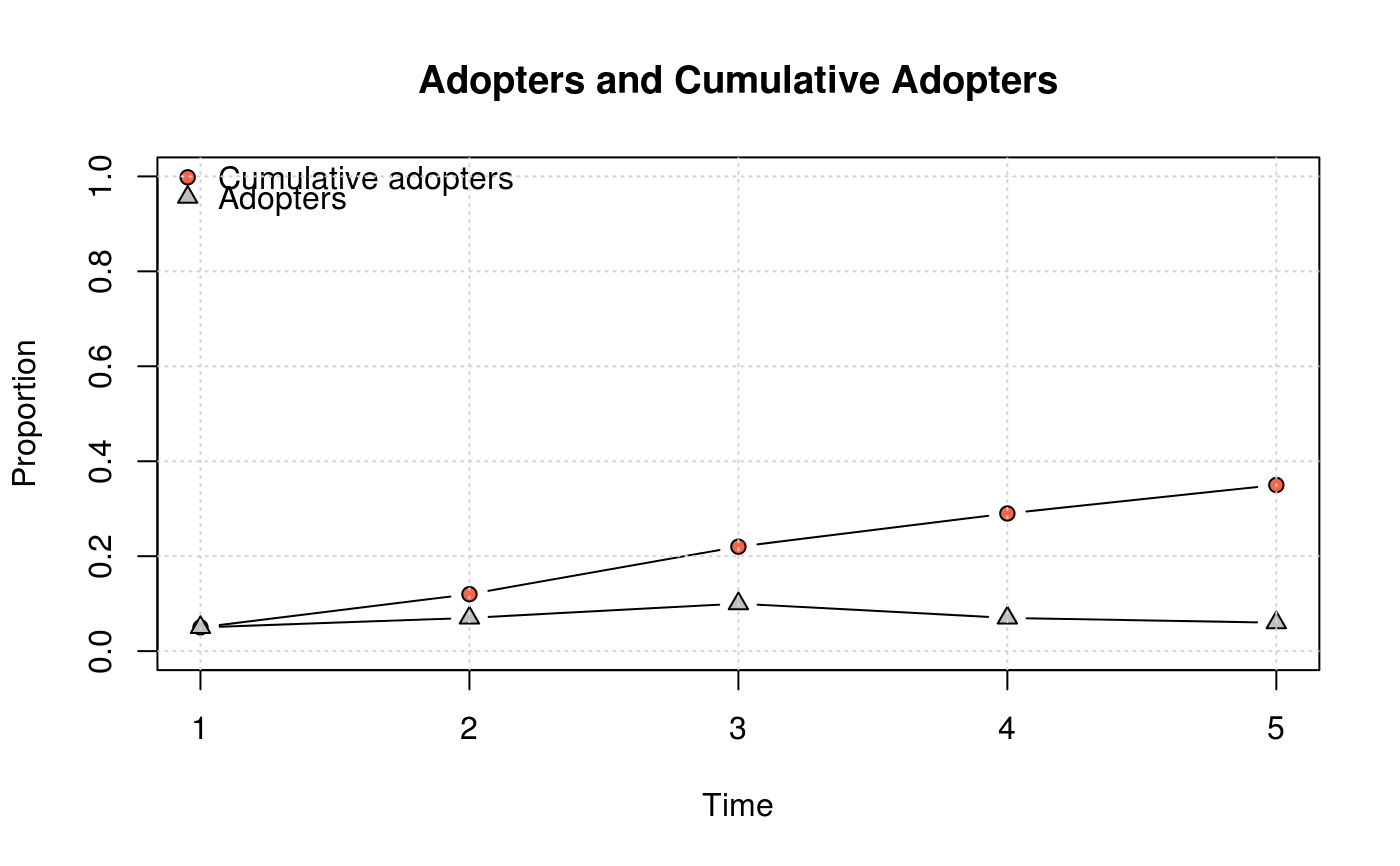
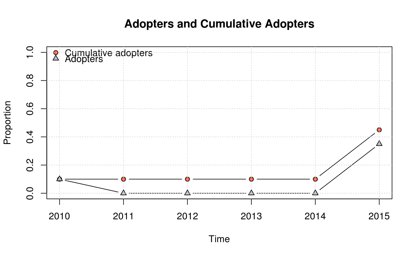
Visualize adopters and cumulative adopters
plot_adopters(
  obj,
  freq = FALSE,
  what = c("adopt", "cumadopt"),
  add = FALSE,
  include.legend = TRUE,
  include.grid = TRUE,
  pch = c(21, 24),
  type = c("b", "b"),
  ylim = if (!freq) c(0, 1) else NULL,
  lty = c(1, 1),
  col = c("black", "black"),
  bg = c("tomato", "gray"),
  xlab = "Time",
  ylab = ifelse(freq, "Frequency", "Proportion"),
  main = "Adopters and Cumulative Adopters",
  ...
)
Arguments
- obj
Either a diffnet object or a cumulative a doption matrix.
- freq
Logical scalar. When TRUE frequencies are plotted instead of proportions.
- what
Character vector of length 2. What to plot.
- add
Logical scalar. When TRUE lines and dots are added to the current graph.
- include.legend
Logical scalar. When TRUE a legend of the graph is plotted.
- include.grid
Logical scalar. When TRUE, the grid of the graph is drawn
- pch
Integer vector of length 2. See
matplot.- type
Character vector of length 2. See
matplot.- ylim
Numeric vector of length 2. Sets the plotting limit for the y-axis.
- lty
Numeric vector of length 2. See
matplot.- col
Character vector of length 2. See
matplot.- bg
Character vector of length 2. See
matplot.- xlab
Character scalar. Name of the x-axis.
- ylab
Character scalar. Name of the y-axis.
- main
Character scalar. Title of the plot
- ...
Further arguments passed to
matplot.
Value
A matrix as described in cumulative_adopt_count.
See also
Other visualizations:
dgr(),
diffusionMap(),
drawColorKey(),
grid_distribution(),
hazard_rate(),
plot_diffnet(),
plot_diffnet2(),
plot_infectsuscep(),
plot_threshold(),
rescale_vertex_igraph()
Examples
# Generating a random diffnet -----------------------------------------------
set.seed(821)
diffnet <- rdiffnet(100, 5, seed.graph="small-world", seed.nodes="central")

plot_adopters(diffnet)


# Alternatively, we can use a TOA Matrix
toa <- sample(c(NA, 2010L,2015L), 20, TRUE)
mat <- toa_mat(toa)
plot_adopters(mat$cumadopt)
