Creates a heatmap based on a graph layout and a vertex attribute
Source:R/plot_diffnet2.r
diffusionMap.RdUsing bi-dimensional kernel smoothers, creates a heatmap based on a graph layout
and colored accordingly to x. This visualization technique is intended
to be used with large graphs.
diffusionMap(graph, ...)

diffmap(graph, ...)

# Default S3 method
diffusionMap(
  graph,
  x,
  x.adj = round_to_seq,
  layout = NULL,
  jitter.args = list(),
  kde2d.args = list(n = 100),
  sharp.criter = function(x, w) {
     wvar(x, w) > (max(x, na.rm = TRUE) - min(x, na.rm
    = TRUE))^2/12
 },
  ...
)

# S3 method for class 'diffnet'
diffusionMap(graph, slice = nslices(graph), ...)

# S3 method for class 'diffnet_diffmap'
image(x, ...)

# S3 method for class 'diffnet_diffmap'
print(x, ...)

# S3 method for class 'diffnet_diffmap'
plot(x, y = NULL, ...)
Arguments
- graph
A square matrix of size \(n\times n\).
- ...
Arguments passed to method.
- x
An vector of length \(n\). Usually a
toavector.- x.adj
Function to adjust
x. If notNULLthen it is applied toxat the beginning (see details).- layout
Either a \(n\times 2\) matrix of coordinates or a layout function applied to
graph(must return coordinates).- jitter.args
A list including arguments to be passed to
jitter.- kde2d.args
A list including arguments to be passed to
kde2d.- sharp.criter
A function choose whether to apply a weighted mean for each cell, or randomize over the values present in that cell (see details).
- slice
Integer scalar. Slice of the network to be used as baseline for drawing the graph.
- y
Ignored.
Value
A list of class diffnet_diffmap
- coords
A matrix of size \(n\times 2\) of vertices coordinates.
- map
Output from
kde2d. This is a list with 3 elements, vectorsx,yand matrixzof size \(n\times n\) (passed viakde2d.args).- h
Bandwidth passed to
kde2d.
Details
The image is created using the function kde2d from
the MASS package. The complete algorithm follows:
xis coerced into integer and the range is adjusted to start from 1.NAare replaced by zero.If no
layoutis passed, layout is computed usinglayout_nicelyfrom igraphThen, a
kde2dmap is computed for each level ofx. The resulting matrices are added up as a weighted sum. This only holds if at the cell level the functionsharp.criterreturnsFALSE.The jitter function is applied to the repeated coordinates.
2D kernel is computed using
kde2dover the coordinates.
The function sharp.criter must take two values, a vector of levels and a
vector of weights. It must return a logical scalar with value equal to TRUE
when a randomization at the cell level must be done, in which case the final
value of the cell is chosen using sample(x, 1, prob=w).
The resulting matrix can be passed to image or similar.
The argument x.adj uses by default the function round_to_seq
which basically maps x to a fix length sequence of numbers such that
x.adj(x) resembles an integer sequence.
References
Vega Yon, George G., and Valente, Thomas W., Visualizing Large Annotated Networks as Heatmaps using Weighted Averages based on Kernel Smoothers (Working paper).
See also
Other visualizations:
dgr(),
drawColorKey(),
grid_distribution(),
hazard_rate(),
plot_adopters(),
plot_diffnet(),
plot_diffnet2(),
plot_infectsuscep(),
plot_threshold(),
rescale_vertex_igraph()
Examples
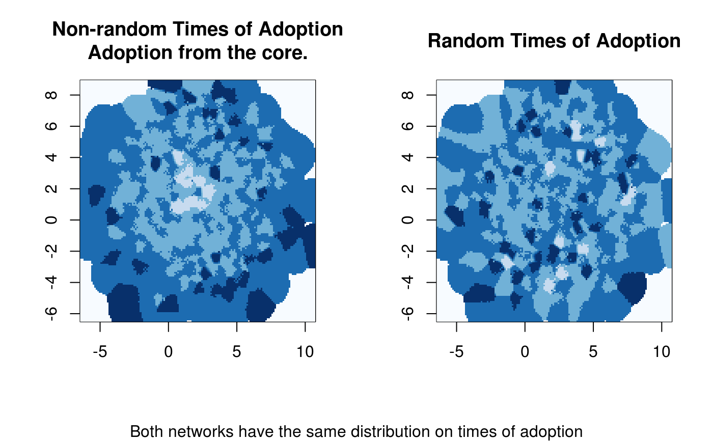
# Example with a random graph --------------------------------------------------
set.seed(1231)
# Random scale-free diffusion network
x <- rdiffnet(500, 4, seed.graph="scale-free", seed.p.adopt = .025,
rewire = FALSE, seed.nodes = "central",
rgraph.arg=list(self=FALSE, m=4),
threshold.dist = function(id) runif(1,.2,.4))
# Diffusion map (no random toa)
dm0 <- diffusionMap(x, kde2d.args=list(n=150, h=.5), layout=igraph::layout_with_fr)
# Random
diffnet.toa(x) <- sample(x$toa, size = nnodes(x))
# Diffusion map (random toa)
dm1 <- diffusionMap(x, layout = dm0$coords, kde2d.args=list(n=150, h=.5))
oldpar <- par(no.readonly = TRUE)
col <- colorRampPalette(blues9)(100)
par(mfrow=c(1,2), oma=c(1,0,0,0))
image(dm0, col=col, main="Non-random Times of Adoption\nAdoption from the core.")
image(dm1, col=col, main="Random Times of Adoption")
par(mfrow=c(1,1))
mtext("Both networks have the same distribution on times of adoption", 1,
outer = TRUE)
 par(oldpar)
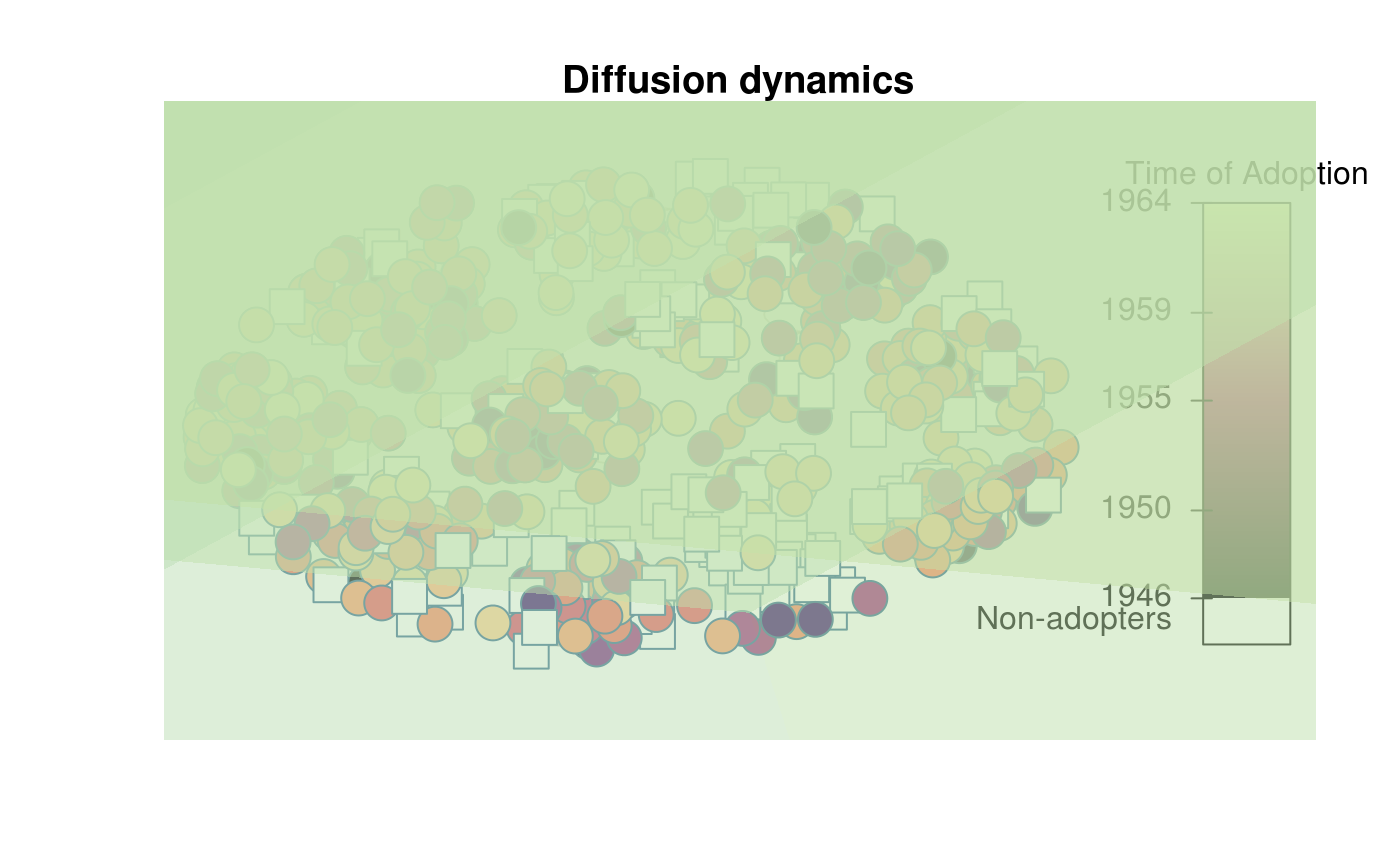
# Example with Brazilian Farmers --------------------------------------------
dn <- brfarmersDiffNet
# Setting last TOA as NA
diffnet.toa(dn)[dn$toa == max(dn$toa)] <-
NA
# Coordinates
coords <- sna::gplot.layout.fruchtermanreingold(
as.matrix(dn$graph[[1]]), layout.par=NULL
)
# Plotting diffusion
plot_diffnet2(dn, layout=coords, vertex.size = 300)
# Adding diffusion map
out <- diffusionMap(dn, layout=coords, kde2d.args=list(n=100, h=50))
col <- adjustcolor(colorRampPalette(c("white","lightblue", "yellow", "red"))(100),.5)
with(out$map, .filled.contour(x,y,z,pretty(range(z), 100),col))
par(oldpar)
# Example with Brazilian Farmers --------------------------------------------
dn <- brfarmersDiffNet
# Setting last TOA as NA
diffnet.toa(dn)[dn$toa == max(dn$toa)] <-
NA
# Coordinates
coords <- sna::gplot.layout.fruchtermanreingold(
as.matrix(dn$graph[[1]]), layout.par=NULL
)
# Plotting diffusion
plot_diffnet2(dn, layout=coords, vertex.size = 300)
# Adding diffusion map
out <- diffusionMap(dn, layout=coords, kde2d.args=list(n=100, h=50))
col <- adjustcolor(colorRampPalette(c("white","lightblue", "yellow", "red"))(100),.5)
with(out$map, .filled.contour(x,y,z,pretty(range(z), 100),col))